Search

Simulistics

Model catalogue

Listed by keyword

Listed by ID

Listed by title

Listed by date added

Lotka-Volterra predator-prey model (Seppelt and Richter, 2005)

Model : predator_prey32
Simile version : 3.x (4.x)
Date added : 2005-09-30
Keywords :

Description

This is a modified Lotka-Voterra model of predator-prey interactions with a prey carrying capacity, K, and a sigmoid predator response function.

This model is provided primarily as a test of Simile's numerical integration methods. It consists of a pair of highly-coupled, non-linear, ordinary differential equations, and is an example of a 'stiff' model, in which the results obtained by simulating model behaviour are sensitive to the choice of algorithm and time step used for numerical integration.

This model was used as the basis for a comparison of the numeric performance of simulation modelling software by Seppelt and Richter, 2005 (reference below). These authors found that Simile did not produce the expected oscillations in predator and prey numbers. However, neither Simulistics nor the authors themselves have been able to reproduce the results published in that paper, and a note correcting the published results is currently (October 2005) in preparation.

Files

Model file Click on the icon to download the model file. (You will need Simile to examine and run the model. A free evaluation version is available from the products page.) Some browsers may attempt to display the model file, rather than open it in Simile; in this case, use the browser back button to return to this page, and use the context menu (invoked by right-clicking on the link) to save the target file to disk.

predator_prey32.sml

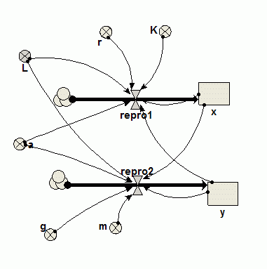
Diagram

Equations

Compartment x : Prey
      Initial value = 10
      Rate of change = + repro1

Compartment y : predator
      Initial value = 0.02
      Rate of change = + repro2

Flow repro1
      repro1 = r*x*(1-x/K)-a*x*x/(x*x+L)*y

Flow repro2
      repro2 = g*y*(a*x*x/(x*x+L))-m*y

Variable K
      K = 1000

Variable L
      L = 50

Variable a
      a = 5

Variable g
      g = 0.2

Variable m
      m = 0.9

Variable r
      r = 0.06

Results

|

a) Results from Simile 3.2, Euler numerical integration, dt=0.1	b) Results from Simile 3.2, Euler numerical integration, dt=0.01
c) Results from Simile 4.4, Euler numerical integration, dt=0.1	a) Results from Simile 4.4, 4th order Runge-Kutta numerical integration, dt=0.1

Note that decreasing the step size when using the Euler integration from 0.1 to 0.01 has a significant effect on the results and so the smaller time step should be used (see What time step should I use?). 4^th order Runge-Kutta is a new feature of Simile version 4 and is more efficient that Euler, note that the results using 4^th order Runge-Kutta with dt=0.1 are close to those obtained using Euler with dt=0.01. |

Web links

Euler numerical integration
4^th order Runge-Kutta numerical integration

References

Seppelt, R. and Richter, O. (2005) “It was an artefact not the result”: A note on systems dynamic model development tools. Environmental Modelling and Software 20(12) 1543-1548

Copyright 2003-2024 Simulistics Ltd