Search

Simulistics

Model catalogue

Listed by keyword

Listed by ID

Listed by title

Listed by date added

Spatial n-state Markov model of vegetation dynamics or land-use change

Model : markov2
Simile version : 3.1+
Date added : 2003-06-25
Keywords : Vegetation dynamics ; Land-use change ; Markov model ; Spatial modelling ; Stochastic modelling ;

Description

Consider an area divided into grid squares, with each square having one of n possible states. These could correspond to n differenttypes of vegetation, or n land uses. There is a certain probability that each state will undergo a transition to some other state, with this probability depending on the current state. Grid squares behave independently of each other.

This model implements a case where there are three states, i.e. n = 3. We thus need a 3x3 array to capture the conditional probability of state i changing to state j during one time step. In the present case, we use the following table:

From \ To	1	2	3
1	0.96	0.02	0.02
2	0.02	0.96	0.02
3	0.02	0.02	0.96

In other words, each state has (in this particular example) a 96% chance of staying the same, and a 2% chance of changing to each other state.

To make this work, we need to be able to randomly generate a state (an integer between 1 and 3) with the correct probability. Thus, if the current state is 1 (the top row), we need to be able to generate a 1 with a probability of 0.96, a 2 with a probability of 0.02, and a 3 with a probability of 0.02.

One way of doing this is to use the “colin( )” function (named after the famous vegetation ecologist, who first presented us with the problem of modelling this situation in Simile). The present example shows another way of tackling it. It works like this:

• Simile can readily generate a random number between (say) 0.0 and 1.0, using the built-in function “rand_var( )”. For the first row in the above table: if the random value is between 0.0 and 0.96, we choose state 1; if it’s between 0.96 and 0.98, we choose state 2; if it’s between 0.98 and 1.0, we choose state 3. These 3 pairs (0.0,0.96), (0.96,0.98) and (0.98,1.0) represent the lower and upper values respectively of the cumulative probabilities.

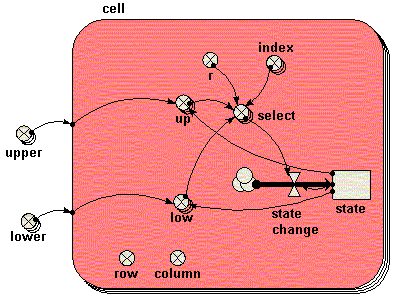
In the present implementation, these lower and upper values are represented in two 3x3 arrays, held in the variables lower and upper respectively. Within the grid cell submodel, one row from these two arrays is selected, according to the current state of that cell. This is then compared with a random number r to determine the new state. This is then used to engineer an appropriate value for the flow causing a change in the state compartment.

Files

Model file Click on the icon to download the model file. (You will need Simile to examine and run the model. A free evaluation version is available from the products page.) Some browsers may attempt to display the model file, rather than open it in Simile; in this case, use the browser back button to return to this page, and use the context menu (invoked by right-clicking on the link) to save the target file to disk.

markov2.sml

Diagram

Equations

Equations in ../Desktop
    upper = [[0.96,0.98,1.0],[0.02,0.98,1.0],[0.02,0.04,1.0]]
    lower = [[0.0,0.96,0.98],[0.0,0.02,0.98],[0.0,0.02,0.04]]

Equations in cell
    state: initial value = 1

    state change = -(state)+sum([select])
    select = if r>[low]and r<[up]then[index]else 0
    r = rand_var(0,1)
    up = element([[upper]],state)
    low = element([[lower]],state)
    index = [1,2,3]
    row = fmod(index(1)-1,20)+1
    column = floor((index(1)-1)/20)+1

Results

|

The following image shows the types of results that are obtained, visualised using the grid display helper. The three colours represent 3 vegetation types.

|

Copyright 2003-2024 Simulistics Ltd