Iterative solution to Ball-Berry stomatal conductance simultaneous equations (Simile V4+)

Model : BallBerry4a
Simile version : 4.0
Date added : 2004-11-25
Keywords : Stomatal conductance ; Evapotranspiration ; Ecophysiology ; Technique ; Iteration ;

Description

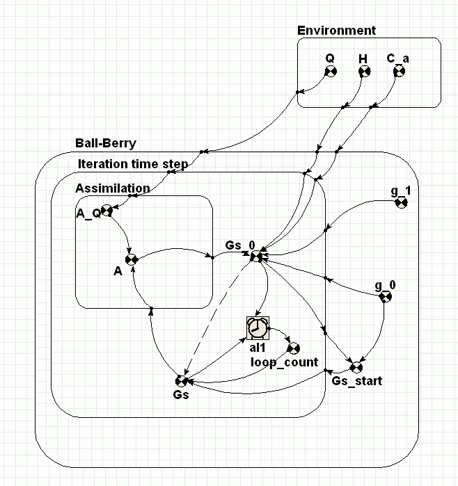
The Ball-Berry stomatal conductance poses a problem for conventional System Dynamics modelling tools because it depends upon the solution of the following pair of simultaneous equations.

Gs = g₀ + g₁ * A * H / C_a
A = Gs * A_Q

Apart from the external parameters, g0, g1, H, Ca and AQ, the equation for Gs depends only on A, and the equation for A depends only on Gs. In this implementation, the loop is opened, by introducing a place-holder for Gs, called Gs_0. This variable is calculated from A. A is calculated using Gs. A guess is made for the initial value of Gs. Subsequently, Gs is set to the last calculated value of Gs_0. The influence arrow from Gs_0 to Gs is dashed, indicating that the value from the previous iteration is to be used. The alarm symbol terminates the iterative loop when Gs and Gs_0 differ by less than one part in one thousand.

That’s all there is to it, except that it’s worth noting what to do if the iteration does not converge. It is necessary to use the new “Abort Execution” command in the “Model” menu of the model diagram window (i.e. NOT in the run control window).

Files

Model file Click on the icon to download the model file. (You will need Simile to examine and run the model. A free evaluation version is available from the products page.) Some browsers may attempt to display the model file, rather than open it in Simile; in this case, use the browser back button to return to this page, and use the context menu (invoked by right-clicking on the link) to save the target file to disk.

BallBerry4aP.sml

Diagram

Equations

Equations in BallBerry4aP

Equations in Environment
 
Variable   C_a : Carbon dioxide concentration (umol CO2 (mol air)^-1)
	C_a = graph(time()) 
	Comments:
		Typical diurnal curve in forest canopy 
 
Variable   H : Relative humidity (proportion)
	H = graph(time()) 
	Comments:
		Typical diurnal graph (24 hour) 
 
Variable   Q : Photon flux density (umol m^-2 s^-1)
	Q = graph(time()) 
	Comments:
		Graph for a sunny day (24 hours) 

Equations in Ball-Berry
 
Variable   Gs_start
	Gs_start = if time()==0 then g_0 else last(Gs_0) 
	Where:
		Gs_0=Iteration time step/Gs_0 
 
Variable   g_0 : Stomatal conductance in the dark (mol m^-2 s^-1)
	g_0 = 0.01 
 
Variable   g_1 : Ball-Berry stomatal conductance coefficient
	g_1 = 23 

Equations in Iteration time step
 
Alarm   
Variable   Gs
	Gs = if loop_count==0 then Gs_start else Gs_0 
	Where:
		Gs_start=../Gs_start 
 
Variable   Gs_0 : Stomatal conductance (mol m^-2 s^-1)
	Gs_0 = g_0+g_1*A*H/C_a 
	Where:
		A=Assimilation/A
		H=../../Environment/H
		C_a=../../Environment/C_a
		g_0=../g_0
		g_1=../g_1 
	Comments:
		Ball-Berry equation 
 
Variable   loop_count
	loop_count = iterations(al1) 

Equations in Assimilation
 
Variable   A : Assimation (umol CO2 m^-2 s^-1)
	A = A_Q*Gs 
	Where:
		Gs=../Gs 
 
Variable   A_Q : Assimilation light response curve
	A_Q = graph(Q) 
	Where:
		Q=../../../Environment/Q 
	Comments:
		Relationship of Assimilation with photon flux density (light) when stomatal conductance (Gs) is maximum 

Results

Copyright 2003-2024 Simulistics Ltd