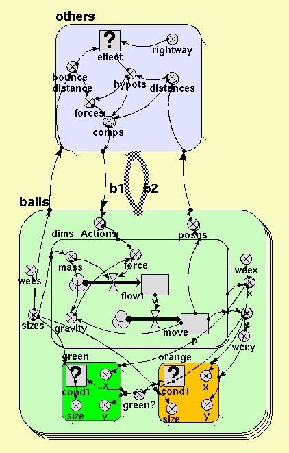
Contained submodel(s)
others
balls
Submodel others
Submodel others is a relation submodel for a relation between balls and itself.
Condition for existence of submodel
effect
Units: boolean
effect = hypots<bounce_distance and rightway
Where:
bounce_distance is the variable bounce distance in this submodel.
hypots is the variable hypots in this submodel.
rightway is the variable rightway in this submodel.
Variable(s)
comps
Units: array(1,2)
comps = forces*[distances]/hypots
Where:
forces is the variable forces in this submodel.
hypots is the variable hypots in this submodel.
[distances] is the variable distances in this submodel.
bounce distance
Units: 1
bounce distance = sizes_b1+sizes_b2
Where:
sizes_b1 is the variable sizes in balls
sizes_b2 is the variable sizes in balls
distances
Units: array(1,2)
distances = [posns_b1]-[posns_b2]
Where:
[posns_b1] is the variable posns in balls
[posns_b2] is the variable posns in balls
hypots
Units: 1
hypots = hypot(element([distances],1),element([distances],2))
Where:
[distances] is the variable distances in this submodel.
forces
Units: 1
forces = pow(bounce_distance/hypots,4)
Where:
bounce_distance is the variable bounce distance in this submodel.
hypots is the variable hypots in this submodel.
rightway
Units: boolean
rightway = index(1)<index(2)
Submodel balls
Submodel balls is a fixed membership submodel with 32 members.
Variable(s)
Actions
Units: array(1,2)
Actions = sum({[comps_b1]})-sum({[comps_b2]})
Where:
{[comps_b1]} is the variable comps in others
{[comps_b2]} is the variable comps in others
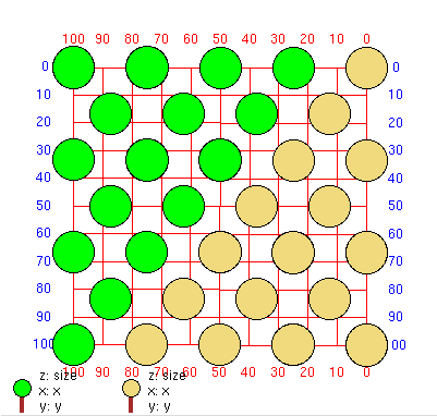
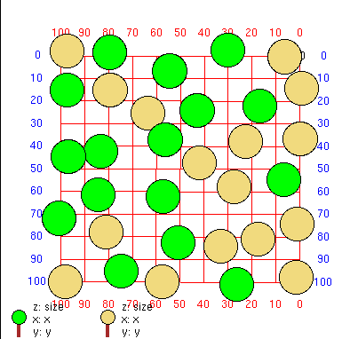
green?
any(index(1)==[2,3,4,5,7,8,9])
Units: boolean
green? = any(index(1)==[2,3,4,5,7,8,9,12,13,14,17,18,22,23,27,32])
posns
Units: array(1,2)
posns = [p]
Where:
[p] is the compartment p in balls/dims
x
Units: 1
x = element([p],1)
Where:
[p] is the compartment p in balls/dims
y
Units: 1
y = element([p],2)
Where:
[p] is the compartment p in balls/dims
sizes
Units: 1
sizes = 15
wees
Units: 1
wees = sizes/10
Where:
sizes is the variable sizes in this submodel.
weex
Units: 1
weex = x/10+45
Where:
x is the variable x in this submodel.
weey
Units: 1
weey = y/10+45
Where:
y is the variable y in this submodel.
Contained submodel(s)
green
dims
orange
Submodel balls/green
Submodel green is a conditional submodel.
Condition for existence of submodel
cond1
Units: boolean
cond1 = green_
Where:
green_ is the variable green? in balls
Variable(s)
size
Units: 1
size = sizes
Where:
sizes is the variable sizes in balls
x
Units: 1
x = x
Where:
x is the variable x in balls
y
Units: 1
y = y
Where:
y is the variable y in balls
Submodel balls/dims
Submodel dims is a fixed membership submodel with 2 members.
Compartment(s)
p
Units: 1
Initial value: if index(1)==1 then fmod(25*(index(2)-1),112.5) else 16.66*int((index(2)-1)/4.5)
Inflows: move
v
Units: 1
Initial value: 0
Inflows: flow1
Flow(s)
move
Units: 1
move = v
Where:
v is the compartment v in this submodel.
flow1
Units: 1
flow1 = force/mass
Where:
force is the variable force in this submodel.
mass is the variable mass in this submodel.
Variable(s)
gravity
Units: 1
gravity = 10*mass*if p<0 then 0-p elseif p>100 then 100-p else 0
Where:
mass is the variable mass in this submodel.
p is the compartment p in this submodel.
force
Units: 1
force = a+element([Actions],index(1))+rand_var(-10,10)
mass
Units: 1
mass = sizes*sizes/100
Where:
sizes is the variable sizes in balls
Submodel balls/orange
Submodel orange is a conditional submodel.
Condition for existence of submodel
cond1
Units:
cond1 = missing
Variable(s)
size
Units: 1
size = sizes
Where:
sizes is the variable sizes in balls
x
Units: 1
x = x
Where:
x is the variable x in balls
y
Units: 1
y = y
Where: