Running models : Working with visualisation tools : Others
Using other helpers
Because of the ease with which new helpers can be developed (see below for details) a great many other helpers exist, alongside the plotter and the data table. These helpers are of a variety of ages and provenances, and do not conform to any consistent interface. Some were developed for specific applications, and although they are of general interest, reflect their origins in their design.
In order to use a helper, your model firstly needs to be built: that is, you need to have selected the "Build" item from the "Model" menu, as described in Running Models. Almost all these helpers work best in the multiple-windows run time environment. The procedure for adding helpers differs, depending on whether the single or multiple-window run time environment is selected.
- in the single-window run time environment, add helpers using the "Add" menu; or
- in the multiple-windows run time environment, add helpers using the "Add tool" submenu in the "IOTools" menu.
The other helpers included in the standard installation of Simile are:
- Plot value against time
- Lollipop diagram
- Spatial grid display
- Polygon diagram (map)
- Sounds for events
- 3d viewer
- Time profiles
With the exception of the "Plot value against time" helper, all these helpers are primarily designed to display data from multiple-instance submodels. The spatial grid display and the three-dimensional viewer are designed to display data from multiple patches of land. The time lollipop display and the time profiles helper are designed to display the attributes of each instance of a population submodel. All these helpers use the following procedure for binding variables.
There are a few other tools, which don't actually perform the input/output functions of helpers but which are implemented as helpers because they operate on the executing model. One is used to initialise the pseudo-random number generator:
 Initialise pseudo-random number generator
Another is used to alter the behaviour of functions defined by sketch graphs:
New to Simile v6: a tool which saves selected model values to file each time step:
Binding variables to helpers
When you select, for example, the "Plot value against time" helper, you need to specify which variable in your model will be plotted. Therefore, the helper issues an instruction, asking you to select a variable by clicking on it in the model explorer or in the model diagram window. Other helpers require more than one variable: in these cases, the instructions indicate the sequence in which the variables should be selected. For example, the "Lollipop diagram" helper (which displays trees in three dimensions) requires you to click first on a variable representing the x-coordinate of each tree; then on one representing the y-coordinates; then on one representing the heights. Note that no checks are made to ensure that the variable you select for x-coordinates really does contain x-coordinates: it is up to you to choose the right one.
Each helper uses one of two methods for instructing you to select the necessary variable(s):
- Separate instruction window: a small window instructing you to click on a model element. The window will tell you the role of the variable that you are selecting in relation to the helper's task, and you need to click on a variable that is appropriate to that role.
- Instructions in the helper window: an instruction about what you should be doing in the helper window itself. One example is the slider input helper. Typically, this allows you to repeatedly select variables from the model, with each one being added to the helper.
Developing new helpers
Simile is probably unique in the world of visual modelling software in that no input/output tools are built into the software. Rather, every such tool is implemented as a separate program in an industry-standard interpreted language called Tcl/Tk. When you load Simile, it creates a list of available helpers by looking in the "IOTools" directory for appropriate files. This is the list of helpers that is then bound into the menus.
One advantage of this approach is that with simple programming anyone can implement a helper customised to their own requirements: there is no need to submit a request to Simulistics (though you are, of course, welcome to do so). This means that if you are modelling (for example) whales, you can implement a display helper that shows whales swimming around. These helpers can be distributed easily, as simply copying the file to the "IOTools" directory is sufficient to install the helper in each copy of Simile.
In: Contents >> Running models >> Working with helpers
Running models : Working with visualisation tools : Grid
Spatial grid display helper
The spatial grid display colours a two dimensional rectangular grid according to the value of a specified variable within each grid square. It is typically implemented using a multiple-instance fixed membership submodel.
Positioning the grid squares
When you add a helper of this type, you are first requested to supply a variable to use as the colimn ids. This variable must have the same number of values as the one that is actually to be displayed, but it is only used to calculate the dimensions of the grid. The grid will have one column for each discrete value in this variable (e.g., if the values are 1,1,1,5,5,9,9,9,9 thenthere are 3 discrete values, 1, 5 and 9). The number of rows will be the total number of values divided by the number of columns. The actual values are unimportant.
You are then requested to supply a variable from which to get the values for the square colours. This variable should have the same number of values as that used to define the columns. If there are more values, the later ones will be ignored. The values are placed in the grid starting at the bottom left corner and going across to the right, then filling the next row from the bottom and so on. If there are fewer values than the number of cells in the grid, they will be used again to fill the rest of the grid.
Zooming and scrolling
The + and - buttons in this helper enlarge and reduce the displayed grid, in steps of one pixel per grid square. When the grid extends beyond the boundaries of the display port, you can use the scrollbars at the borders to bring various parts of it into view. Note that the colour legend will always obscure part of the grid if you can scroll perpendicularly to it. To see all of the grid, you can move the legend between the bottom and the right of the display using the "Orientation" radio buttons in the helper's properties dialogue. The 'Save' button will save an image showing the legend and visible part of the grid, in the format indicated by the supplied file extension.
Choosing colours for values
The legend shows which colours correspond to which values from the variable. It has different colours over a certain range of values. The range can be increased or decreased with the < and > arrow buttons in the toolbar, or it can be set exactly using the "Scale range" entry fields in the properties dialogue. If the data variable is boolean or enumerated type, there will be one colour for each of its possible values. If it is an integer, there will be a different colour for each value in the range, up to 100 colours. Otherwise, there will be 33 colours corresponding to smaller ranges of values within the whole range. Values outside the range are shown in the colour for the nearest end of the range.
For numerical values, there are initially three colours for low, middle and high, (black, yellow and white in the image above) with other colours fading between these for other values. This arrangement can be changed using the colour map editor.
Viewing and changing information
The grid display normally updates as the model runs, but can be frozen by clicking the "Freeze" button at the right of the toolbar (this feature is left over from the days when the graphics took a long time to update; these days they are very fast).
Clicking on the display gives a popup with the column and row number of the grid square in which you clicked, plus its value (which will be approximate if the display is using colours to represent ranges of values). Dragging produces more poups for each grid square entered. Hovering over a colour in the legend shows what value it represents.
The grid helper can also be used to set the values of model parameters. This does not work for variables other than parameters. Click on the "enter edit mode" button (with the pencil icon) then click on the colour legend to select a colour to "paint" onto the grid. Click on the legend again to paint a new colour. Changes made to parameter values in this way will not take effect immediately; the same rules apply as for changes made with the slider helper.
Saving information as GeoTIFF
The second tab in the properties dialogue allows the grid to be saved as a GeoTIFF (for more information see section on loading GeoTIFF data). To use this tool you must have the GDAL library installed on your computer. Load a template file from which to copy the georeferencing data, then save a new file using the data from the grid. This is useful if you have parameterized your model with data from GeoTIFF files. You can also choose to have a file saved at each display interval after the grid data is updated; the time value will be appended to the chosen filename.
A three-dimensional view of a rectangular grid is also possible using the 3d viewer.
In: Contents >> Running models >> Working with helpers
The Colour Key Editor
Simile can now produce displays of grid or polygon data with a wide choice of colour keys thanks to the colour key editor. It is possible to reproduce the sort of colour keys typically used in relief maps, thermographic imaging systems, weather maps and magnetic surveys. The colour key editor can be invoked from most visualization tools that can express data as colour.
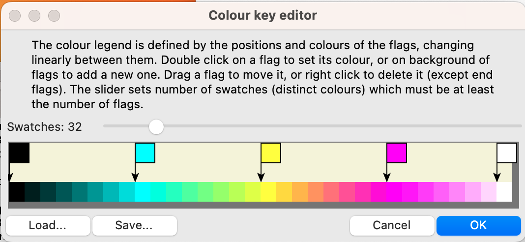
As well as editing the key as described in the dialogue, it can be loaded or saved in .rgb format, which is widely used by GIS systems. Simile's examples directory contains a saved legend, 'eightbit.rgb', which generates swatches corresponding to the colours that would be converted into each integer between 0 and 255 when using the 'eight-bit colourmap' option in the image data loader. It is thus possible to view an image which was loaded as data in a grid helper, possibly after it has been altered by execution of the model.
Running models : Working with visualisation tools : Plot value
Plot value against time helper
This is the classic time-plot helper. For most uses, it has been largely replaced by the Plotter helper.
It was not designed for presentation in a printed document, but for giving the model developer a robust, flexible display of how the value(s) for a single variable change over time. It automatically re-scales, on both the X (time) and Y axes, it can handle a variable no matter how deeply nested in multiple-instance submodels, and it displays the results from previous runs for comparison. It also gives the current values for all the variables in text form.
Each time you select a "Plot value against time" helper, you need to choose the variable to be plotted before the helper is displayed. You are alerted to this requirement by the message:
The following screen dumps show the standard ways this helper can be used.
This shows the value for a single-valued variable "size" from three successive runs of the model, using different parameter settings on each run. Note the automatic use of a different colour for each run, and the current value displayed at the bottom-left.
This shows the set of time plots for a single variable embedded inside a fixed-membership multiple-instance submodel. Since the number of instances is fixed for the duration of the run, we have the same number of lines throughout. Note that the line for each instance is different, reflecting the fact that each instance has different parameter values even though they all behave according to the same equations.
Here again we have the plot for a single run, for a single variable embedded inside a multiple-instance submodel. This time however the submodel is a population submodel, with individual instances coming into existence and disappearing during the course of the simulation run. Note then how lines start during the simulation (unlike the previous example, when all lines started at time zero), and also terminate during the course of the simulation, as individual instances are killed off. Each line has a different slope, reflecting the fact that the model was set up with a randomly-determined parameter value for each instance.
In: Contents >> Running models >> Working with helpers
Running models : Working with visualisation tools : Profiles
Time profiles helper
The time profiles helper is designed to show multiple attributes of each
instance of a population submodel. Each instance must be assigned a unique
identifier, which is plotted sequentially on the y-axis. A stacked bar
chart display is used to plot an arbitrary number of properties of that
instance against time.
For example, each individual in a population may hold wealth in the form
of property, stocks and shares, and cash. The time profiles helper will
display the changing wealth of each individual over time (the total height
of each bar) as well as the make-up of that wealth (the height of each
coloured segment).
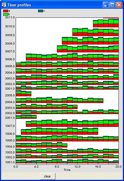
For best results, the variables plotted should be scaled to be less than
50. Panning and zooming operations are implemented as for the plotter helper. The y-axis can be panned up or down and
the x-axis panned left or right to display different parts of the axis at
the same magnification, whilst both axes can also be zoomed in or out to
increase or decrease the magnification.
-
 The cursor takes on the shape of a
four-headed arrow when placed over a scale point. Dragging a scale point
alters the range displayed by zooming in or out. To zoom in, drag the
scale points away from the origin, i.e. to the right (on the x-axis) or
upwards (on the y-axis). To zoom out, drag the scale points towards the
origin, i.e. to the left (on the x-axis) or downwards (on the y-axis).
-
 The cursor takes on the shape of a
two-headed arrow when placed over the axis itself. Dragging the axis
alters the range displayed by panning up or down, left or right.
In: Contents >> Running models >> Working with helpers
Running models : Working with visualisation tools : Model Explorer
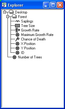
Model Explorer
The model explorer provides a nested tree view of all the variables, compartments and flows used in the model. The elements are arranged by submodel, hierarchically from the top level desktop. In variable-membership submodels, additional elements used only in those submodels are also displayed. When a "helper" window requires a variable to be selected, this action can be performed by clicking on the required variable in the model explorer.
In: Contents >> Running models >> Working with helpers
Running models : Working with visualisation tools : Lollipop
Lollipop diagram helper
The "Lollipop diagram" is a means of displaying tree-like objects distributed in two dimensions. Each object has a size, which is used to calculate both the length of the trunk and branches. After invoking the helper, three variables are required for each component whose values are to be displayed, corresponding to the x-coordinates, the y-coordinates and the sizes. These can be variables or compartments, and are typically in a multiple-instance submodel. One tree then corresponds to each instance of the submodel.
Each set of values is displayed as trees of a diferent colour. A horizontal grid is also drawn, with x positions numbered in red, and y positions in blue. Numbers corresponding to heights of trees (z variable in the legend) are positioned above the grid corners in black.
There are sliders to adjust the longitude (view angle) and latitude (view elev.) of the point on an imaginary sphere surrounding the grid from which it is viewed. The image can be printed.
Note that all three variables can change through time, so although real-world trees may not move, their graphical representations can. This means the lollipop diagram helper can also be used for simulating animal movements, and so forth.
For best results, the x- and y-coordinates should be scaled between 0 and 100, and the size should be less than 25.
In: Contents >> Running models >> Working with helpers
Running models : Working with visualisation tools : Initialise
Standard helpers: Initial pseudo-random number generator
The functions rand_var() and rand_const() generate random numbers. For greater understanding of model behaviour it is sometimes convenient to generate the same (or the same sequence) of random numbers for several model runs. To do this, it is necessary to seed the random number generator with the same integer value each run. For this reason, they are known as pseudo-random numbers. A simple tool is provided to enter the seed.
To enter the seed:
- enter an integer value in the edit box;
- click on the "Set seed" button; and
- reset the model.
Note: It is important that the ![]() reset button on the "Run Control" is used AFTER initialising the pseudo-random number generator using the "Set seed" command. This is because some random numbers are generated when the model is reset.
reset button on the "Run Control" is used AFTER initialising the pseudo-random number generator using the "Set seed" command. This is because some random numbers are generated when the model is reset.
Example
Using the seed "123" will produce the following sequence of random numbers for the function rand_var(0,100) every time the simulation is performed:
62.3463, 2.2889, 13.6723, 11.7893, 92.8648, 56.7217, 93.8688, 96.4232, 96.3378, 75.1671, 49.0097, …
(At least if you are using the bundled MinGW C compiler under Windows. Other compilers may produce different sequences, owing to using different library implementations of the pseudorandom sequence generators, but this tool can still be used to achieve repeatability.)
In: Contents >> Running models >> Working with helpers
Running models : Working with visualisation tools : 3d
3d viewer helper
The 3d viewer helper is similar in operation to the spatial grid display helper, though four variables, rather than two, are required, to display the grid in three dimensions. These are, as before, the x-coordinates and the colours, but also, the y-coordinates and a sizes. Again, these are most commonly implemented using a fixed membership multiple-instance submodel.
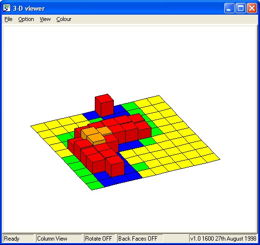
Amongst the many menu options, is the ability to switch to a surface view of the grid, as shown in the following screen shot. There are also options to rotate the graph through three dimensions, and to select the colours used.
In: Contents >> Running models >> Working with helpers
Other visualization tools : Event sounds helper
Other visualization tools : Event sounds helper
The motivation behind Simile's visualization tools is to provide the modeller with a continuous, immediate understanding of what the model is doing. Sometimes the best way to do this is with sounds rather than graphics. With the addition of discrete events to the modelling language, we realized that their instantaneous nature does not lend itself to the kind of graphical displays that work for continuous values.
So we created an event logger that also produces a sound each time a selected event occurs. Add an instance of this tool in the standard way, selecting 'Event sounds' from the list of helper titles. Now after clicking '+' in the helper window's toolbar, you can select a discrete event component in your model, and a sound file to play each time the event occurs. The window will show a 'ticker bar' which will move across the screen right to left, with a vertical line added each time the event occurs. Hovering over the lines will pop up the exact time and magnitude of the occurrence they represent.
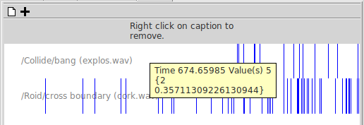
Also, the sound will be played each time the event occurs. If your event has a numeric magnitude, then the volume of the sound will be determined by where each event's magnitude falls between the min and max values given for the event. Sound files in WAV format will play on all platforms -- files in other formats (e.g., mp3) may play on your particular platform but are not guaranteed to play on all.
If the chosen event occurs very frequently, or if it is in a simple model that runs very fast, the sounds may overrun each other producing unpleasant noise. In this case you can use the 'limit updates/sec' feature to slow the model execution down to the point where the sounds can be heard separately.
Running models : Working with visualisation tools : Polygon diagram
Polygon diagram
This tool enables a dataset to be displayed as the colours of polygonal areas on a map. It can be used either where vector data for an actual map is available (either in the model, or in a separate file), or where an area is represented as some regular set of shapes whose vertices can be calculated by the model, e.g. hexagonal tiling.
A lot of the functionality of the polygon helper, including scrolling and zooming, working with the colour legend, and using it to edit model parameter values, is exactly the same as for the grid helper. However, the graphics of the polygon helper are not quite as fast, so you are more likely to need the 'freeze display' and 'manual update' features.
Loading co-ordinates from file
If you choose this option you will get a file selector to locate the data for the coordinates. If you choose a file with the extension .dxf, Simile will attempt to load it as a DXF file, and will then colour the polygons in the order in which they are defined in the file. Otherwise, Simile currently expects the file to contain all the X coordinates in nested list form, followed by all the Y coordinates. This is not particularly convenient, so we should add the option to set the coordinates from file using the table data dialogue too.
Loading co-ordinates from model
Of course you can put fixed parameters in the model and load them using the table data dialogue, then use them to set the boundaries of the polygons. If you choose this option, you will be asked to select model elements representing the X and Y coordinates of the polygon vertices. These elements should have two-dimensional data arrays, with the outer index being the number of the polygon whose border they define, and the inner index being the number of the vertex around that polygon. There should be the same number and arrangement of X and Y coordinates.
The usual way to get the coordinates is to have a submodel for the vertices inside the submodel representing the polygons. This should be a per-record submodel if different polygons have different numbers of vertices. Put fixed parameters for Xs and Ys inside the vertices submodel.
In: Contents >> Running models >> Working with helpers
Running models : Working with visualization tools : Edit sketch graph function
Standard helpers : edit sketch graph function
If your model contains equations that use the graph function, their function can be altered while the model is running. The tool for doing this appears as a helper, although it does not display values from the model or directly set them.
The helper is located in the "Standard tools" subdirectory menu and is called "Edit sketch graph function". Create an instance of the helper and click on the model component whose function you wish to alter. You will then see the same sketch graph editing window as when you originally created the sketch graph. You are able to drag the sketch line as well as edit the axis values and change the settings that control how the sketch is interpreted.
Any changes you make to the sketch graph function will take effect as soon as you hit the 'OK' button, but the helper will stay up until you delete it, allowing further changes to be made at any point. Note that the edited function will not be saved with the model. If you save the model after editing the sketch using the helper, it will keep the original version of the function. To change this you must go back to the equation dialogue and hit the "Graph" button.
Running models : Working with visualization tools : Data logger
The Data Logger tool does not display model data, but records it in files for later analysis with statistical tools. There are other ways of doing this:
- The Table Helper can save its contents as a .csv file, but has poor performance with large data sets
- The Snapshot tool can record values as the model runs, but only handles one variable, and needs setting up every time the model is run
By contrast, the Data Logger can handle any size of data set that is usable within Simile, and can log multiple variables, either in separate files or as columns in a single file. Since it is a standard helper, many instances can be added for different groups of values, and the setup can be saved as part of a general helper layout.
Using the tool
The tool's canvas will be blank when it is first added. To log a variable, hit the + button and click the variable on the model diagram. It will be listed within its hierarchy of submodels, with a '-' button ffor its removal. Hit + again to add more variables. The rightmost button in the helper's toolbar switches between saving separate files for each variable (named by the variable's caption) and a single file (log.csv) with each variable in its own column.
Saved file format
The helper will not save any data until you select a folder in which to save it. Click the toolbar button with the folder icon and navigate to the desired location. Now a line is written to the log file(s) at each display point as the model executes. The files are in .csv format with the time points stored in the left hand column. If the values being saved are arrays, they will be written as series of alternating indices and values, with each series enclosed in curly brackets, i.e., the same format as data popups or directly-entered file parameters.
The file is closed when the model is paused, and opened for appending more data when it is restarted. When the model is first run after a reset or rebuild, the file will be opened for writing, so the previous contents will be overwritten unless they have been moved.
As of Simile v6.9, it is also possible to log model data to a database -- either a file in some Excel-compatible format (.xls, .xlsx etc) or a MySQL database. To log to a database file, simply select it from the file dialogue. To log to a MySQL database, cancel the file dialogue and this will cause the database specification dialogue to appear. Here you enter the hostname, username, password and name of the MySQL database.
When logging to a database, each component being logged will have values put in its own column in the database. If logging an array component, there will be a separate column for each element in the array, named value/n where value is the name of the component and n is the index of the element. (value/n1/n2/... for multi-dimensional arrays). The values will be written to a table called 'Run 0' until the model is reset, after which new tables called 'Run 1', 'Run 2' etc will be created for data values from subsequent runs.
In: Contents >> Running models >> Working with helpers