Running models
Running models
Once you have drawn the model diagram and specified how to calculate the value of each element, you are ready to perform a simulation. During the simulation, the model is run for a specified number of time steps, and the changing values of any of the elements can be plotted, recorded in tables, or displayed using a variety of other visual tools. You can develop your own displays specific to the needs of your models.
Preparing models to run
Before it runs a model, Simile generates an executable program from the model diagram.
Diagnostic messages
How Simile interacts with the modeller to display and correct problems
Run time environment
Simile provides two alternative environments for running models and seeing the results of the simulation. The standard one uses a single window containing a number of panels: one for controlling the simulation, another for any input sliders, and others that can contain graphs or other ways of visualising model behaviour. The alternative, multiple-window environment has a separate window for each of these.
You decide which of the two run-time environments you want by ticking or un-ticking the option "Single-window Model Run Environment" in the Preferences dialogue window, obtained by selecting the Preferences item in the Edit menu.
As of Simile v6.12 it is possible to have a browser window display the status of the running model.
Controlling model execution
Whichever execution environment you choose, you control the model's execution via the run control panel. This is either a special box within the single execution window, or a whole window itself, but looks the same in either case. It allows you to:
-
start, pause and reset the model's execution,
-
set the time for which it will execute and the frequency of display updates, and
-
adjust other execution variables such as the step size and integration method.
Visualising model behaviour
The term "helper" is the generic term in Simile for any tool for displaying model behaviour (i.e. the values for variables), or for entering values into a running model.
Parameter estimation and predictive analysis
Simile incorporates an interface to the PEST parameter estimation tool. This carries out parameter estimation by varying model parameters in order to match model behaviour with measured data from the system being modelled. It can generate prediction ranges for model outputs based on combinations of parameter values found in this way.
Working with external data
If your model has variables whose data source is chosen as being from file, i.e. so-called "file parameters", then it requires data to be provided before the simulation can proceed. A file parameter dialogue window will appear to enable you to provide the required information.
Scripting model execution
In addition to the interactive run-time environments, a scripting interface is provided to enable simulations to be run without user interaction. This is often useful for simulation experiments, e.g. running the same model for a set of scenarios (probably defined by parameters in a scenario file), for sensitivity analysis or parameter estimation.
In: Contents
Running models : building models
Running simulations : preparing a model for running
Simile runs a model by executing a program that it has generated specifically for that model. This program contains all the instructions need to calculate the values of the model variables as they change over time. Whenever you want to run the model after making any changes to it, you must re-generate this program. At the same time, the value of all the variables are calculated ready for the start of the simulation.
To build the model, select either the "Run" command in the Model menu, or the "Debug" command. These generate programs in either of two languages, C++ or Tcl, respectively. Use the "Debug" command if you have a problem running your model, due to a mathematical error. You will get a more informative error message. Otherwise, use the "Run" command, for faster model execution.
If you use the Windows or Mac versions of Simile, you may choose to use a c++ compiler already installed on your computer rather than the one included with Simile. The Preferences dialogue window, obtained by selecting the Preferences item in the Edit menu, is used to indicate which C++ compiler is to be invoked. An open source C++ compiler, GNU g++, is included in the Simile distribution. Under Windows, Microsoft Visual C++ is also supported. Linux users on the other hand are expected to have the GNU g++ compiler installed on their system, and Simile will always use this compiler.
Development of a model will often involve an "edit/run cycle" in which the modeller alternates between exploring the behaviour of the running model, and making changes to the model diagram and equations. Changes to the model diagram and equations are not reflected in the behaviour of the executing model until "Run" or "Debug" is selected again. Interacting with an executing model that is out-of-date will produce a warning message and a change in the status indicator. This warning message provides an option of rebuilding the model, and there is also a "rerun" button in the model window toolbar (play arrow or running man) that rebuilds the model and starts it running in a single operation.
In: Contents >> Running models
Running models : diagnostic dialogues
Running models: diagnostic dialogues
The point at which you attempt to run a newly built model is where you are most likely to encounter failures due to incompleteness or inconsistencies in the model's definition. You should not give up at this point; a bit of attention to the messages will enable the problems to be fixed.
The first dialogue that appears will have an outline description of the problem, and only two buttons. Depending on the nature of the problem, these can be:
- OK / More info...
The problem has stopped whatever task was in progress from being completed. You can hit "OK" to go back and try again, or "More info..." to see a more detailed message, and get a reference to these help pages where appropriate.
- Give up / See all...
The task in progress can continue, although it will not be successfully concluded. You can hit "Give up", fix the indicated problem and try again, or "See all..." to keep running the task and display a list of all the problems found at the end.
- Default option / More options...
There are several possible actions that can be taken at this point. The most frequently chosen is named on the left button, while the right button opens another dialogue displaying all the options.
Errors during model building
These are problems that come up during the process of converting the Simile model to code that can run on the computer. There are many possible causes, the simplest being that not all components have their values specified (i.e., they are still red). Other building errors can arise if a component has been specified correctly, but its specification does not make sense in its context in the model, often because the context was changed after the component was edited. Several of these messages include useful information to help fix the problem, for instance:
Problem building code, e.g., Simile failed to convert var1 (in submodel submodel1) into a program instruction.
Something like this means that the component has an equation, but it no longer fits the component's place in the model. If you hit 'More info', then 'See full error text', you will see the error you would get if you tried to enter the same equation for the component now (or else you can just do so!). For instance, the parameter names that can be used in the equation might have changed, or a submodel index might no longer be valid.
Problem with model design, e.g., This model cannot be executed because it contains the following circular set(s) of function evaluations: [var1,increment(var2_sum),var2_sum,var2,made_for(var1,var2,1)]
Here, no one component is wrong, but the model cannot be built because together they do not make sense. In this case, a set of influence arrows form a circle, so there is no sensible order in which to evaluate the components they join together (see rules for using influences). The error message includes a list of all the components that form the circular chain, plus other entries representing intermediate steps performed by Simile in evaluating components.
Problem during compilation of model code
Simile has managed to convert the model into executable code, but the compiler (a separate program that turns c++ code into binary instructions) is having none of it. This usually means that there is a bug in Simile which is causing it to generate incorrect c++ code. The only thing you can do is file a bug report including your model code to Simulistics. However a compilation error is also triggered by an explicit division by zero, since the compiler will not build binary code that inevitably gives bad results. In that case you can rebuild your model using the 'debug' menu entry to find the location of the division-by-zero expressed in terms of model components (i.e., which component, in which submodel).
Problems linking model with parameters or visualization tools
These can occur either when a new helper setup or parameter file is loaded while a model is running, or if a model is changed and rerun while keeping the same helper setup or parameters. It means the component names listed in the file no longer exactly match the components in the model.
For example, the above is the "Some parameter values unused" dialogue. If a parameter metafile contains parameterization information relating to components that do not exist in the model you are trying to run, you have four options: Discard values (the default: ignore values for the missing component and keep loading the rest of the data), Give up, Use elsewhere (find a model component with a different name that can take the values for the missing one) or see help. The initial dialogue offers only the "Discard values" option and "More options...". Choosing the latter brings up the dialogue displayed above.
The Use elsewhere button is useful in the case where you have changed the name of a model component or a submodel containing it, or added or deleted a submodel boundary around it, since saving the parameter metafile. In the case above, the dialogue is pointing out that some parameters are for a component in a submodel that no longer exists in the model. In this case, hitting Use Elsewhere will bring up a tree diagram showing all the submodel captions in your model, and their nesting relation. When you select a submodel from this list, Simile will try to find the components from the lost submodel in that submodel instead, and supply the parameter data to them. If this works, you should re-save the parameter metafile later to avoid having to do the same thing again next time you open the model.
Problems during model execution
e.g., "Simile ran into a problem trying to run this model.
While calculating the value of {external procedure} during execution of the model at time 1275.0, there was an OS signal: 11 (SIGSEGV)."
These messages relate to problems in a model's logic that only become apparent when the model is running. These occur because some of Simile's advanced features require that the modeller stick to certain rules when using them, or else something undefined will happen in the model. The most commonly used such features are:
- The element() function. The second argument can be an expression, but it must always evaluate to a number between 1 and the number of elements in the array that is the first argument, otherwise it will attempt to get a value that does not exist.
- Dashed influences. These allow a model containing a circle of influences to be executed, specifying that the component at the head of the dashed influence can be evaluated without waiting for the one at the tail. But its equation should contain something like an 'if' clause to insert a boundary condition in any case where the tail does not already have a value anyway.
- Base instance lookup. While Simile will not allow a base instance lookup if the index is out of range, it is possible to cause other problems with this feature, for instance by looking up multiple base instances in the wrong order, e.g., any(index(1) is [10, 5, 1]).
When an error like this occurs, the model cannot continue to run. If it happens during reset or initialization, the execution LED goes grey and the model must be rebuilt before it will run again. If it happens during execution, the LED goes red and the model can be reset and run again. However, in either case, if the same problem occurs again, Simile will crash.
To get more information about the cause of these bugs, run the model using the 'debug' menu entry. This causes the model to be built and run in a scripting language, where attempts to access undefined values will produce a list of procedure calls from which Simile can deduce what actually was missing in the model. Here's an example:
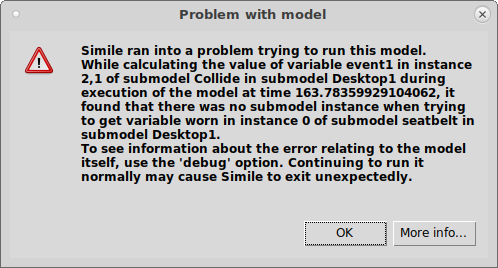
Here we can see the name of the variable in whose equation the error occurred (event1), the name and indices of the submodel instance containing it (Collide) and so on up to the desktop, and the identity of the missing quantity (the variable "worn") and why it failed (it was looking for the value from the instance of its parent submodel "seatbelt" with index 0 -- the index of the first element is 1). The message about using the debug option is irrelevant -- to get this level of detail, the modeller must already be using it. There are similar messages if the variable itself is missing, for instance due to unprotected use of the dashed influence, or a bad index for an array variable.
In: Help >> Running models
Running models : Single window run time environment
The single-window Model Run Environment
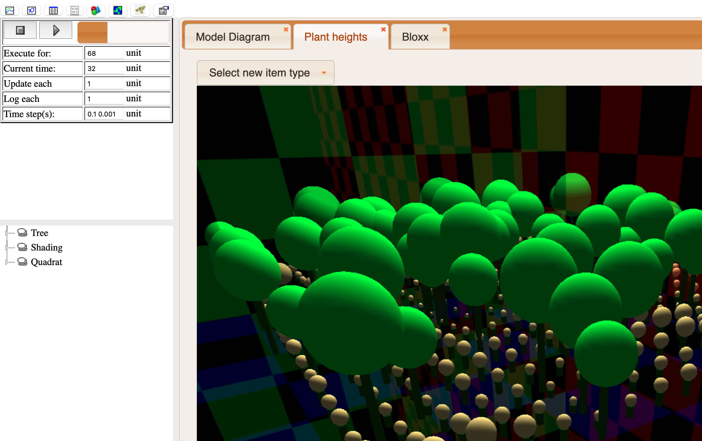
Controlling a simulation and displaying results is performed within the Model Run Environment (MRE). The single-window MRE provides flexible self-contained access to all the controls needed to perform a simulation and to display the results.
It is divided into a number of sections. In the upper left corner is the "Run Control". In the lower left corner is a tabbed panel containing the model "Explorer". On the right hand side are four notebook pages, which can each contain one or more "helpers". Helpers are used to display the behaviour of a model whilst it is running, for example, a graph of a variable, or a data table. Helpers are also used to provide data for the model, for example, using "Input sliders".
To add a helper to a page, select the required helper from the "Add" menu. The three most commonly used helpers can be selected using these buttons on the tool bar:
 the plotter;
 the data table; and
 the Input sliders.
The pages can be divided vertically or horizontally, to allow more than one helper to be display on each page, and pages can be added or removed. Once one or more helpers have been added to the pages, and are arranged as you wish, the configuration can be saved to a file, for use the next time the same model is built.
- To save the current configuration of helpers, chose the "Save configuration…" item on the "File" menu, or use the
 save button on the tool bar.
 - To load a previously saved configuration of helpers, chose the "Load configuration…" item on the "File" menu, or use the
 open button on the tool bar.
 - A
 new configuration can be selected, to remove all the currently displayed helpers.
Arranging pages, and panes
|
|
Add notebook |
Creates a new notebook, initially with four pages, in the current pane |
|
|
Add notebook page |
Adds a page to the notebook containing the current pane |
|
|
Divide pane vertically or horizontally |
Splits a pane into two new ones separated by a sash which can be dragged |


Adding helpers
|
|
Add plotter |
|
|
Add table |
|
|
Add sliders |
|
|
Add other helper |

Manipulating layout
|
|
Copy display to clipboard |
Copies helper window to Simile's clipboard; also copies its graphics to system clipboard for pasting into other graphical applications |
|
|
Cut display to clipboard |
As above but also removes helper window from the pane |
|
|
Paste display from clipboard |
Inserts a copy of the helper window from the clipboard to the current pane, with the same setup |
|
|
Delete display or helper |
Removes helper window from pane, or deletes pane if it is already empty |
|
|
Print display contents | Prints the graphics of the helper in the current pane |


Saving and restoring configurations
|
|
New configuration |
Sets MRE to its initial state of one notebook with four empty pages |
|
|
Open configuration |
Loads a previously saved configuration. Model components referred to by the helpers in the configuration should exist in the current model. |
|
|
Save configuration |
Saves a configuration for reloading later, or for inclusion in a model package. |
In: Contents >> Running models
Running models : Working with visualisation tools : Save and restore
Helper configurations
You will probably be working with a particular model over a period of time, testing it, modifying it and exploring its behaviour. Often, you will want to have the same displays each time you run a simulation. Simile enables you to save a particular configuration of helpers in a file, and re-load them on a subsequent occasion.
Each configuration can contain one or more instances of one or more types of helper, each instance linked up to particular variables in the model. You can have several configurations for the same model. You can also use the same configuration for different models - perhaps slightly different versions of one model - so long as the variable names are the same. For this reason, configurations are stored in separate files, and not in the file used to save the model itself.
 New configuration
Any existing helpers are closed and removed by selecting a new configuration. It is only necessary to name the configuration when saving it, in which case any suitable name and directory can be chosen in the usual way.
 Save configuration
The procedure for saving configurations differs, depending on whether the single or multiple-window run time environment is selected.
- in the single-window run time environment, save configurations using the "Save configuration" item on the "File" menu; or
- in the multiple-windows run time environment, save configurations using the "Save" item in the "IOTools" menu.
 Load configuration
The procedure for loading configurations differs, depending on whether the single or multiple-window run time environment is selected.
- in the single-window run time environment, load configurations using the "Load configuration" item on the "File" menu; or
- in the multiple-windows run time environment, load configurations using the "Load" item in the "IOTools" menu.
In: Contents >> Running models >> Working with helpers
Running models : Multiple window run time environment
The multiple-window Model Run Environment
The multiple-window Run-Time Environment uses a separate window for the dialogue windows and displays concerned with running the model. There are the model diagram window, the Run Control, Sliders (if required) and helpers. Helpers are used to display the behaviour of a model whilst it is running, for example, a graph of a variable, or a data table.
In the multiple-window Run-Time Environment, the display helpers are selected from the "I/O Tools" menu of the model diagram window. Each time one is selected, another window is created, plus (in some cases) instructions for selecting the variables which are to be displayed by the helper. To remove a helper, close its window. Note that the "I/O Tools" menu appears only when a model has been built.
Note that this Model Run Environment is provided mainly for compatibility with earlier versions of Simile, and will be phased out with the release of Simile v7. Some old helpers may only function effectively in this environment, for example. Otherwise, the new single-window Model Run Environment should prove more flexible and convenient.
In: Contents >> Running models
Running models : Running in browser
Running in browser (Simile v6.12 on)
If this option is selected, then instead of a run control window appearing as part of the Simile user interface, a new browser window or tab will be created to show the model run status. This looks similar to the SimiLive web interface, and actually downloads some code from the SimiLive server in order to operate, but the model data is coming from the local Simile which will be acting as a web server.
If the option is selected when the model is already running using the Simile single-window run interface, then then that Simile window will be hidden and the browser page will be layed out according to the layout of visualization tools previously in use, i.e., with the same set of notebook tabs and the same panes and display tools visible in each tab. There will be an extra notebook tab showing the model diagram, complete with equation and value tooltips over the model components. Switching to and from execution in the browser causes the model to reset. Further visualization tools can be added using the tool buttons in the browser page. However these changes are lost when going back to running the model in Simile's own run environment.
This mode of model execution is useful for previewing how model execution will look if it is to be published for use via SimiLive. Also, the 3-D shape viewer in browser execution is implemented in WebGL and produces fully rendered displays, which look a lot better than the displays in Simile's own shape viewer, and also has better performance rendering complex scenes.
Running models : Run control
Run control panel
The run control panel is a notebook containing two tabs. The first of these, headed 'Run control', is the one usually displayed, and provides the most commonly used actions for controlling the execution, as well as indications of progress. The other tab, 'Run settings', gives access to selections which fine-tune the model execution, and will not usually be displayed.
Run control tab
The run control is used to start and stop the simulation of the model.
-
the
 play button will begin execution at the current time for a number of time steps set using "Execute for".
 -
the
 stop button will stop the simulation (if one is running) and set the current time to zero.
 -
the
 pause button will pause the simulation at the current time.
Note that the pause button is only displayed if a simulation is running, and the play button is only displayed if one is not.
The progress bar indicates the elapsed time as a proportion of the total. To the right of the progress bar is an LED which changes colour to indicate the current status of the simulation. This table explains the meanings of the most commonly seen LED colours.
|
LED colour |
Corresponding model status |
|---|---|
|
|
Model is stopped and ready to run |
|
|
Model is stopped and ready to run, but has been edited since the execution was started so the results might not correspond to the current model diagram |
|
|
Model is initializing, resetting or loading data from file parameters |
|
|
Model is executing |
|
|
Display tools are busy updating their images |
|
|
The model has been stopped, either by executing the stop(...) function, or by a mathematical error, and needs to be reset |
|
|
The model code is loaded but some fixed parameter values must be supplied for it to run |
|
|
The model has been stopped by a program error, and the executable code needs to be rebuilt |
 Black
Black Purple
 Yellow
 Green
Green Blue
Blue Red
Red Grey
Grey White
WhiteDuring a long run, the LED may appear some shade between green and blue; this can be interpreted as indicating what proportion of time Simile is spending actually executing the model as opposed to redrawing the displays of the visualization tools. From version 5.4 onwards, Simile is capable of running the model and updating its displays simultaneously when running on a multi-CPU computer; the LED is blue while doing both at once.
The other fields on this tab are:
-
Execute for
This setting controls the number of time units for which the model is run each time you push the "play" button. You can enter a negative number here to use your model for backcasting, i.e., extrapolating the past from the present.
-
Current time
This setting displays the current number of elapsed time units. It is possible to enter a value into this field, if you wish to begin a simulation at some time other than zero. Note, however, that unless your model contains events that occur at some pre-defined time, this is unlikely to make any difference.
-
Display interval
During the course of a simulation run, each helper extracts values from the model for whatever variables it is displaying. This happens at an interval determined by the value in this field. The display interval is specified as a fraction (or multiple) of the time unit. The display interval cannot be shorter than the shortest time step. Setting a short display interval will cause fast-changing values to be displayed with more detail, but will slow down execution of the model.
Starting with version 6.0, there is a checkbox to the left of the display interval field, labelled 'event;' if this is checked, the state of the display tools will also be updated whenever a discrete event occurs in the model. This is particularly useful in two cases: where values of events are being recorded, since an event only has a value at the exact point in time at which it occurs; and when an event causes a change in direction of a continuously varying component, in which case this option allows a graph point to be added at the exact position of the direction change.
-
Time step
The time step for a simulation model is the fraction of the unit of time at which all variables are updated within the model. For example, imagine a model consisting of a single compartment which is initially empty, and a flow into the compartment at a rate of 2 litres per day. In this case, if the unit of time is set to be the day, and a time step of 0.1 days is chosen, then Simile will calculate the change to the compartment every 1/10th of a day. Thus, after the first time step, the container would contain 0.2 litres, i.e. 1/10 of 2 litres, 0.4 litres after the next time step, and so on. After one day (ten time steps) the compartment will contain 2 litres.
Run settings tab
The following actions are available on the second tab of the run control panel:
-
Select time units
This setting is for use with physical units, to specify the particular time unit, rather than using abstract time units. If you have not specified consistent physical units for all flows, you should not change this setting from the default "unit". If you have specified consistent physical units, you should choose the unit you wish to use to specify how long to execute the model for.
-
The integration method determines how the update of state variables is calculated on each time step. If your model uses Systems Dynamics elements only (i.e. compartments, flows and variables) then you will find Runge-Kutta to be more accurate with less computational effort. For all other models, Euler integration will be more reliable. Please see the page on Runge-Kutta integration for more details.
-
Some problem domains have behaviour that alters between slow, steady changes and rapid fluctuations. These are known as 'stiff systems' and one way to model them accurately is to use adaptive step size variation. What happens is that the model execution monitor makes an estimate of the integration error after each time step, and if it is greater than a certain limit, it reverts the model to the state it was in at the start of that time step and re-does it as two time steps of half the duration. The error estimation and reduction process is repeated for each of those time steps, but if a very low error value is estimated after the second of two equal steps, the time step returns to its previous longer value before execution continues. The value entered in the Time step field is now the maximum length of a time step.
To enable adaptive step size variation, check the box to the left of the word "Adaptive;" and enter a suitable error limit in the entry box to the right. Note that the error limit is used as an absolute value, so models with large numerical values will tend to be run with shorter time steps than those with small numerical values. This changes with Simile v5.7: the error sensitivity now depends on the difference between the user-supplied minimum and maximum values for the compartment (see Equation Dialogue). The larger this difference, the less sensitive the step size will be to integration errors for a given compartment. If either the minimum or maximum value is not specified, it will treat the difference as 100, which results in the same behaviour as for earlier Simile versions.
-
Simple models run very, very fast in Simile. This may not always be desirable, for instance if one is trying to control an ongoing simulation in real time by using a slider, or if trying to stop it in response to some event. So it is possible to limit the frequency at which model time steps are executed. To do this, check the box to the left of the label "Limit updates/sec to:" and enter your maximum update rate to the right.
-
Time at reset
Normally, the model time after reset is zero. However, it is sometimes useful to have the model time set differently at reset, for instance if the model's initial state relates to a historical date and it is parameterized with a time series that is indexed by subsequent dates. In this case, the time units may (or may not) be set to Year, and 'time at reset' set to a given year, so the model time corresponds to the calendar time in the domain being simulated. This will also result in the X axis of graphs, etc, being annotated with values that can be read as the calendar time.
-
If an occurrence type is selected here, the model will pause whenever that thing happens. The preferences dialogue includes an option that decides whether a dialogue will be displayed when this happens. In any case an entry will be added to the Log tab, describing what happened, and the model can be restarted by hitting the 'Play' button again. The occurrence types are events (which does not include time series events) and compartment under/overruns. If this is selected, the model will pause every time a compartment goes below its minimum or above its maximum value, as set in the equation dialogue. This can be useful for debugging models.
Log tab
This tab contains a list of descriptions of things that happen while running the model, including events and compartment under/overruns if they are selected (see above), and user-defined pauses. The contents of the log tab are formatted as a table with fields enclosed in curly brackets, and can be cut and pasetd into other applications, e.g., spreadsheets.
Further notes
What display interval should I use?
When choosing a display interval, bear in mind the following factors:
-
If it is very small, then you will slow down the simulation. Updating the display is relatively time-consuming, and the smaller the display interval, the more frequently this happens.
-
If it is too large, you may miss important dynamics, especially in a simulation that shows sudden swings in behaviour. An extreme case of this is when you are simulating switching behaviour: for example, in simulating overflow of a container with fixed capacity by allowing an overflow to operate when the contents of the container exceeds a maximum. In this case, you may get a very misleading graph for the overflow (perhaps showing extended periods of no overflow followed by extended periods of an overflow). If you do obtain apparently aberrant behaviour, then set the display interval to be the same as the time step, so that you are quite sure that you are seeing exactly what is happening to the variable.
Observing the proportion of time that the LED status indicator is blue will give you an idea of how important it is to choose the optimum display interval. If the status indicator is blue most of the time you will be able to improve the performance significantly by increasing the display interval. If it is green most of the time, increasing the display interval will have little effect.
Time steps
If the processes that you are simulating in your model are truly continuous, then you are actually specifying a model based on differential equations, with compartments corresponding to state variables. In general, digital computers cannot solve such models exactly, so they resort to various numerical methods for calculating the value of the state variable forward through time. There is a large numbers of such methods, with some of them producing far greater accuracy for a given amount of computational effort than others. Simile uses the simplest such method, the Euler method. The reason for this is that, in general, a Simile model can contain features that make it unsuitable for solving through other, more advanced, numerical methods.
What time step should I use?
There is no simple answer to this question. If the processes you are modelling happen on a discrete-time basis - for example, animals reproducing once per year - then you can use a time step of 1. Otherwise, explore the effect of reducing the time step. If you get no significant difference in model behaviour, then use the bigger time step. If you do get a significant difference, then keep on reducing the time step until you cease to get a change in behaviour.
A useful rule-of-thumb is that no state variable should change by more than two parts in one hundred over one time step.
Why is the time step labelled as being "Time step #1"?
Different submodels in a model can be specified as operating on different time steps (in the submodel properties dialogue). For example, you might have a model with a human demographic submodel operating on an annual time step, and a lake pollution submodel operating on a 1/100th of a year basis. In that case:
Time step #1 = 1
Time step #2 = 0.01
How does adaptive step size variation work?
Simile's adaptive step size variation mechanism differs from other implementations. How it works is, at the end of a time step, a compartment's rate of change is calculated and compared with what it was expected to be when its value at that time was calculated. In the simple case of Euler integration, a compartment's value is calculated with the assumption that its rate of change stays the same throughout the time step, so the estimated error is the difference between the new rate of change and the previous one, times the current step size. Error estimation for Runge-Kutta integration works in a way analogous to this, but the estimated rate of change is a function of the intermediate rates of change generated during the application of that method.
Back-casting
Entering a negative number in the "Execute for..." field in the Run Control enables certain back-casting calculations to be performed. Time will obey the usual rule of stepping from the "Current time" (which you can enter) in steps of magnitude given by "Time step" for the total number of units specified by "Execute for". For example, you could request execution for 100 time units, enter a current time of -100, and a time step of 0.1. Simile will then perform as it usually does by default with 1000 calculations, but in reverse.
In the model equations, you have entered "Initial values" for the compartments (state variables). When the model is first built, or subsequently reset, the "Current time" is set to zero and the compartments are allocated these initial values. Even if the "Current time" is manually changed after this, the compartment values are not changed. It is therefore not possible to enter time-dependent initial values in the model. On the other hand, if you want to enter "Initial values" that represent the state of the system at some non-zero time, this can be achieved by altering the "Current time" setting after the model is built or reset.
If, however, the model is not reset, then the state variables will retain their values from the end of the previous run. This allows a model's calculations to be repeated in reverse, simply by reversing the sign of the time step. (This is a good check on the numerical accuracy of the solution: if the initial values are not re-calculated exactly at the end of the reverse calculation, then the difference is equal to double the error.)
Note: Only models consisting of System Dynamics elements only can reasonably be treated in this way. If population submodels are used, it is not possible to reverse the action of the population control elements through time.
This works with both Euler and Runge-Kutta integration, and given the restriction above, it can usually be assumed that Runge-Kutta integration is preferable.
In: Contents>> Running models
Running models : Using Runge-Kutta integration
Runge-Kutta integration
Runge-Kutta integration provides more accurate values for a given level of computational effort than Euler integration, for those models involving only systems of differential equations. Simile always uses Euler integration by default, because it is applicable to any model.
For example, consider the equation dy/dt = t, and given y = 0 at t = 0. In this case, there is an analytical solution, y = ½t2, and therefore at t = 100, y = 5000. Using the Euler integration algorithm, and using a step-size of 0.1 (the default) Simile calculates the answer to be 4995. Using Runge-Kutta integration, the correct answer of 5000 is found using the same step size (and therefore approximately the same computational effort). Even using a step size of 0.01 the answer is calculated to be 4999.5, using Euler integration.
However, it must be noted that Runge-Kutta integration is not always applicable, unlike Euler integration, which can be used to solve any system of differential or difference equations.
In particular, Simile allows the construction of difference equations, where certain quantities accumulate in sudden increments corresponding to weeks, months or years, for example. Interest payments, in particular, correspond to this method of accumulation. These systems must be solved by Euler integration, with the step size chosen to correspond to the periodicity.
Furthermore, although Runge-Kutta integration does not fail when used with discontinuous functions (such as are involved in the creation and destruction of instances of population submodels) the results will be no more precise than using Euler integration.
The choice between Euler and Runge-Kutta integration is made at run time, using a drop-down box in the Run Control. The chosen method is saved with the model and restored when the model is loaded. The user can experiment with running a model using either method, without having to rebuild the model, to understand whether a significant improvement is achieved.
In: Contents >> Running models
Running models : Working with visualisation tools
Working with helpers
A helper is a tool that can be used to interact with a simulation. Simile provides helpers to display the results of a simulation, for example, to plot graphs, or tabulate data, or to enter data into a simulation as it proceeds. Some helpers do both: for example, the grid display helper also enables the user to set a value for any grid square. It is simple to add new helpers to Simile. If you are interested in learning how to develop new helpers for your own models, please contact us at Simulistics.
Most of the helpers are used as follows:
- If using the Single-window Model Run Environment, select or create an empty pane
- Add a helper tool, either by clicking that helper's button in the MRE toolbar or by selecting it from the pull-down menu ("Add..." or "I/O Tools" -> "Add...")
- Specify which model variables will drive the display, by clicking on them either in the model diagram or in the Model Explorer tool
-
If the tool can display multiple data items, hit the + button to add further items to the display.
Extra features common to several helpers:
- Clear the display with the
 clear button
 - Remove a data item from the display with the - button (values already displayed for it may persist)
- Add notes to the display area of canvas-based helpers (e.g., plotter, grid display) with the T text button
- Configure the helper with the
 configure button
Simile comes provided with a number of standard helpers. Some are generic, such as the "Plotter" and "Data table" helpers. Others are quite domain-specific - the "Lollipop diagram" helper, for example, was developed for displaying tree growth - but are included because (with a little imagination) they can be applied to a range of situations.
 Using the Plotter helper
 Using the Data table helper
 Using the Layered helper (Simile v6.1 and on)
 Using the 3-D Shapes helper (Simile v6.5 and on)
 Using the Slider helper
- Using other helpers
The configuration of helpers best suited to viewing a particular model can be saved to a file.
In: Contents >> Running models
Running models : Working with visualisation tools : Plotter
Plotter helper
The plotter helper is for plotting graphs of one or more variables against time. If a variable has many values, e.g., one in a multiple instance submodel, all the values will be plotted. Different colours are used for different variables, and for data from successive model runs. Hovering over a trace on the diagram will result in a popup window giving the indices of the particular value it represents, the time in the run at which that point was plotted, and its value at that time and at the current time.
 Clearing the display
To remove all the plotted data, click on the ![]() button.
button.
Selecting elements to plot
One or more elements can be added to the graph.
- to add an element, click on the
 button. An instruction is then posted to click on the model element to be plotted. This can be on the model diagram or in the model explorer.
- to remove an element, click on the
 button. An instruction is then posted to click on the element to be removed, in the legend of the graph. Data already plotted for that element will not be removed untiil the clear button is clicked.
Highlighting a trace
Clicking on one of the traces will highlight it by drawing it in double thickness. You can highlight many traces at once. Clicking on it again will reset its display state to normal.
In: Contents >> Running models >> Working with helpers
Running models : Working with visualisation tools : Table
Data table helper
The data table helper is a tool for tabulating the results of a simulation run. You can use it if you want to inspect the simulation results in more detail than you can on a graph, or if you want to export the results, as a data file in comma-separated value (CSV) format, to data presentation or analysis software, e.g. Microsoft Excel.
You can specify as many model variables as you want. Any of the variables can be nested in multiple-instance submodels to any depth, in which case each instance of the submodel will be allocated one column. The leftmost column displays the times at which the values were recorded. Columns can be removed, if desired, after the simulation has completed. The precision (number of decimal places) to which the numbers are displayed can be increased or decreased before each run of the simulation.
Note that for very large arrays of values this tool can run quite slowly, because it is oriented towards interactive display. It can be improved by turning off updating at every display time (this option is available in the properties dialogue). If you want to save very large data sets, or time series from long runs, it may be quicker to use the snapshot tool.
 Clearing the display
To remove all the tabulated data, click on the![]() button. This preserves the column headings, but removes all the rows of data except those corresponding to the current time.
button. This preserves the column headings, but removes all the rows of data except those corresponding to the current time.
Choosing elements to tabulate
The elements to be tabulated are selected as column headings. The procedure for choosing elements is as follows:
-
to add an element, click on the
 button. An instruction is posted, to click on the element to be tabulated. The element can be chosen from the model diagram or from the model explorer.
-
to remove an element, click on the
 button. An instruction is posted, to click on the column headings to be removed. The first click indicates the start of the range of columns to be removed, the second click indicates the end of the range. If the same column is selected twice, only that column is removed.
 Saving table data
To save the data displayed in the helper, click on the Save button. The table will be saved in .csv format with the headers and values arranged as they currently appear in the display. Where headers are spread over more than one column, empty fields will be added to the saved table so that subsequent headers in the same row still line up with the correct data columns.
 Arranging the layout
The layout of the table is controlled using the Table properties dialogue box. Clicking on the Properties ![]() button will bring up a dialogue box with two tabs. These tabs provide options to change the table layout, and to alther the way in which values are displayed.
button will bring up a dialogue box with two tabs. These tabs provide options to change the table layout, and to alther the way in which values are displayed.
Adjusting table layout:
This allows the user to designate which dimensions of the data to use as row and column headings. For example, time can be used as either a row or column heading, and element names and element indices can be used similarly. This tab also includes the option to show current values only as an alternative to showing values for all time points with the relevant time as a row or column heading.
Adjusting value display format
This tab, titled "Variable formats", provides several options for adjusting the way in which values are displayed in the table. The pulldown menu at the top allows you to specify which values the changes made here should apply to; the default is "All" but you can choose to re-format the values of only one particular variable in the table by selecting its caption here.
The leftmost listbox allows you to select the type of value which is being displayed. As opposed to pure numeric values, you may choose to display them as angles (d °m ' s ") with conversion from radians if appropriate, or dates/times with conversion from Julian days. Boolean is provided in case your data uses numerical values to represent true/false states, but if the value is actually boolean in the model, this will be selected by default.
The next listbox allows you to select from a variety of formats for each value type, most importantly between General and Scientific (exponential) for numeric values. The right frame allows the number of decimal places displayed to be adjusted via a spinbox, and provides an option to highlight negative values by displaying them in red as in accounting ledgers.
Logging data over time
Normally, the table helper shows data from the model at any time point corresponding to start of a display interval. By selecting "current values only" from the layout tab, the helper can be made to display only the values for the start of the current display interval. No time heading or time values will appear. In this mode you can unselect "update at display intervals" on the same tab, which results in the data not being updated at all except when the ![]() update button is clicked. When a time axis is displayed, the data is still logged even when it is not updated in the table, so clicking the update button will result in all the values since it was last clicked being displayed.
update button is clicked. When a time axis is displayed, the data is still logged even when it is not updated in the table, so clicking the update button will result in all the values since it was last clicked being displayed.
In: Contents >> Running models >> Working with helpers
Running models : Working with visualization tools : Layers
Layer display
The layer display tool differs from Simile's other display tools in that it allows a number of different types of display to be superimposed to create a composite image of processes in a 2-D modelled world. When the layer display is selected, a blank window appears in the run environment, and the 'Add' menu is replaced by a 'Layers' menu which allows the modeller to add instances of layer tools to the display, and to manipulate existing layers.
There are currently four different layer tools:
- Spatial grid map
- Polygon map
- Input pointer (Simile v6.12 on)
- Background photo
- Moving individuals
As of Simile v6.9 there are also a set of '2-D shapes' tools, for adding layers consisting of circles, lines or ellipses. These are analogous to the corresponding object types in the 3-D Shapes tool.
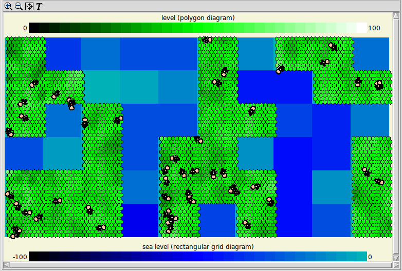
The spatial grid and polygon maps are similar to the corresponding stand-alone spatial grid and polygon tools, with the exception that they cannot be used to change values of model components. The background photo tool simply allows an image to be displayed behind anything that is added by the other tools, and the moving individuals tool displays icons (specified as series of Tk canvas drawing commands) for members of a submodel which includes values representing their co-ordinates in a 2-D space.
Layers menu
When the layer tool is first added, the layers menu will consist of a single entry labelled "Add new layer here". This cascades to a set of menus listing the available layer tools according to their source, like the menu for selecting the regular helper tools. Once a layer tool is added, the modeller will be prompted to select files and/or click on model components whose values will control the layer display, after which the layer will be added to the display. The layers menu now has a new entry for this layer, with 'Add new layer here' entries above and below it.
Once layers have been added, the menu lists all the existing layers, with 'Add new layer here' entries above, below and between them to allow new layers to be added at any position in the stack. Selecting the entry for an existing layer cascades to options to move the layer to the top or bottom of the stack, up or down one level, delete it or open its properties dialogue. A layer's properties dialogue will have a set of input widgets, some of which are unique to the layer type, and some common between various layer tools. The common ones are:
- Select colours: This allows the colours representing the different model values (as shown in the legend) to be changed.
- Range: The range of values covered by the colour spectrum can be widened or narrowed.
- Offset and scale: Normally, data with the same numerical X and Y coordinates will display at the same point in the window in any layer tool, but these values adjust the display position of each layer. They can be used to compensate for different coordinate units being used in different parts of your model, or to show different maps side by side in the same window.
- Legend side: For tools that can display a legend, this selects at which side of the window it appears, if at all. If multiple legends are added to the same side, the ones for the higher layers will be drawn on the inside.
In: Contents >> Running models >> Working with helpers
Working with visualization tools : Layers : Spatial grid map
Spatial grid map
This layer tool is very similar to the spatial grid display, with a couple of exceptions:
- It cannot be used to set the values of model components
- If used with a component in a hexagonal grid, the cells will be shown in a 'brickwork' pattern corresponding to the centres of the hexagons.
This tool may also be slower than the spatial grid display, since a more complex image scaling operation is required to get the grid to the exact scale to match other components.
In: Contents >> Running models >> Working with helpers >> Layer tool
Working with visualization tools : Layers : Polygon map
Polygon map
This layer tool is generally similar to the polygon helper, and is set up in a similar way. The differences are as follows:
- It can be set to redraw the polygon outlines at each display interval, to cope with models in which polygons appear and disappear, or change shape
- It cannot be used to set values of model components
- The value for the colour is selected first. If this is from a hexagonal grid submodel, there is no need to provide vertex coordinates -- the helper generates the hexagon outlines itself.
- The properties dialogue allows a stipple pattern to be chosen for filling the polygons. This allows lower layers to be partially seen through them.
This tool is faster than the old polygon helper with large numbers of polygons.
In: Contents >> Running models >> Working with helpers >> Layer tool
Working with visualisation tools : Layers : 2-D Shapes
2-D Shape Layer
This layer tool is similar to the stand-alone 3-D shape viewer, but displays 2-D shapes in a layer rather than projected 3-D shapes. Whereas one instance of the 3-D shape viewer can display sets of shapes corresponding to several sets of model valriables, each instance of the shape viewer layer only displays a set for one group of model variables. If multiple sets of shapes are required, each one can be added in the same view as a separate layer.
The shapes that can be added are circle, ellipse or line. Each has a separate submenu entry for adding it, so once it is added, the modeller is prompted for the information that enables the display to be set up. X and Y co-ordinates are set from components in the model, or fixed numeric values can be entered in an input field. If a model component is chosen for the colour of a shape, the colour legend editor appears in order to record how the model values will be converted into colours for the corresponding components.
Working with visualisation tools : Layers : Spatial input layer
Spatial input layer
This layer helper allows spatial input to be sent to a model during execution. When it is added as a layer, the modeller is requested to select three variable parameters from the model. These must be scalar with numerical units.
The first two of these will hold the X and Y coordinates of a position in the field of view of the layer tool. They are not changed until the modeller clicks or drags within the tool. At that point they will be continually updated with the pointer position within the layer tool until the unclick. The final variable is set to zero at any time when a click or drag is not in progress. It is set to 1 when a click occurs and is incremented by 1 whenever the pointer coordinates change during a drag. This is so the model can keep track of the speed or duration of the drag. It is set to zero again on the unclick.
This tool does not itself display anything within the layer helper area. Normally it would be added to a layer tool which is also showing a spatial grid covering the area in which the coordinates could be expected to fall, so the tool could be 'zoomed to fit' resulting in the input pointer layer also extending over the right range of coordinates. If there is no actual grid to display, the area covered by the input tool could be set by adding four 'line' layers, each with a single line corresponding to one side of the rectangle containing the desired input coordinates. These coordinates could be entered directly to the layer tool as numbers, or got from model variables.
Working with visualization tools : Layers : Background photo
Background photo
This is not really a visualization tool at all -- it just allows an image to be displayed as a background to the layers. Generally the image will be some form of map that corresponds to the data in the model. Because the pixel pitch of the image may not correspond to the position data in the model, the properties dialogue allows an offset and scale to be set for the image display. Thus the tool also allows the whole layer display to be annotated with small images.
When the tool is selected, a file selection dialogue appears for choosing the image file, which immediately displays. Its offset and scale are then adjusted via its properties dialogue. To change the image, delete the layer and add a new one.
In: Contents >> Running models >> Working with helpers >> Layer tool
Working with visualization tools : Layers : Show moving individuals
Show moving individuals
If a model includes a group of submodel instances representing mobile individuals, it may be desirable to display them on a map background using icons. That is what this layer tool is for. It can draw a lot of copies of an icon representing an individual at positions specified by model data. It can also vary the size and orientation of the icons according to data from the model.
The image data file
In order to do this, the icon must be expressed as a series of canvas drawing commands in the Tk language. Tk is the standard graphics extension for scripting languages including Tcl, Perl, Python and Ruby. An example file to draw the ants in the image on the Layer tool page is included in Simile's examples directory, and the images for Simile's population channels are also encoded in this way. These files typically have the extension .cnv. It is hoped to offer a Paintbox-style drawing tool for creating images in this format in the near future.
The file consists of a series of commands to draw the icon on a canvas referred to as $c. This will cause it to be drawn in the layer display when sourced by this tool's code. If the ability to rotate the icon is to be used, then only canvas objects that can be drawn at any angle should be included, i.e., avoid arcs and ovals (unless circular) and rectangles. As well as drawing commands, the file should include an instruction to set the hotspot -- this is the point in the image that will be positioned on the map point given by the model data, as a pair of integers, e.g.,
set hotspot {100 150}
Similarly the scale should be set, i,e., the number of canvas units of the drawing commands corresponding to one unit of map space. A large value will mean the image is drawn small, and is useful for precision because positions and line thicknesses in the image file must be integers.
set scale 10
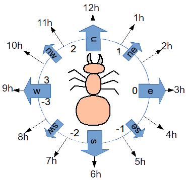
It should also set the axis direction, in which the image as drawn by the canvas commands appears to be facing. This can either be a compass point (ne, sw, etc), an hour on the clock face (6h, 9h, etc) or a number which will be treated as the number of radians the axis lies anticlockwise from the x axis. e.g., these three forms are valid and equivalent:
set axis n
set axis 12h
set axis 1.57
Setting up the tool
When the layer is selected, a file selection dialogue appears for choosing the image file. Once the file is selected, its contents are loaded into the helper setup, so the file is not consulted again -- if the image is altered, the layer must be deleted and re-created to display the new version of the image. Now you will be prompted to click on model components for the x and y coordinates of the individuals' positions on the map. These have to be supplied. You will be prompted to click on two more model components to specify the size and orientation of the individuals. If you do not wish the icons to be changed in size, just click on one of the components you have already clicked on at this point, and the size will not be altered. The value of the orientation component can be a number, which is interpreted as the number of radians anticlockwise from the x axis which the image will be shown facing. Alternatively it can be a member one of the enumerated types used to index the neighbour directions in the special-purpose submodels, in which case the image will be drawn facing in that direction. In either case, if the value of the direction component is the same as the axis direction in the model file, the icon is drawn unrotated. If no rotation is to be done, select a component that has already been selected for x or y position as the rotation.
In: Contents >> Running models >> Working with helpers >> Layer tool
Running models : Working with visualization tools : 3-D Shape Viewer
3-D Shape Viewer
This is another helper that can superimpose shapes representing information from a number of different model components which may represent different types of object and have different array dimensions. In this case, a set of model components can be used to provide data for a shape or group of shapes in a 3-D scene. For instance in this representation of a plant, a sphere is used to show the root volume, cylinders are used to show the leaf stems (petioles) and ellipses are used to show the leaves themselves.
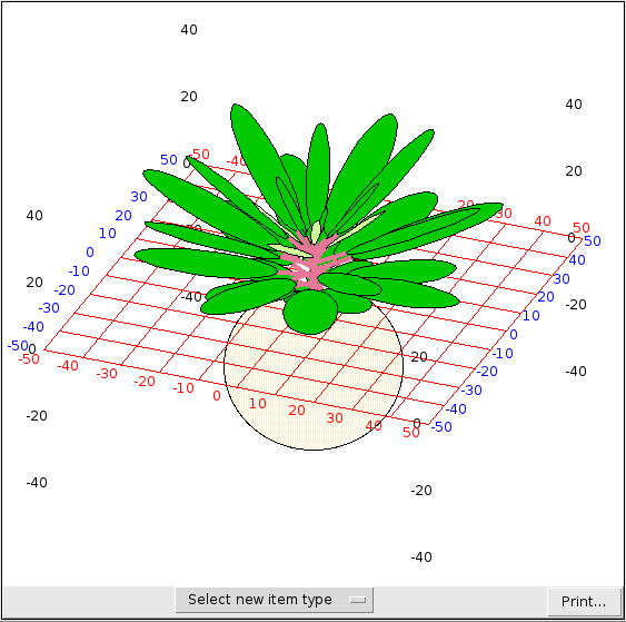
When the helper is first invoked, the grid is displayed showing X axis indices in red, Y in blue and Z in black. There are currently three types of shape which can be added. The dimensions of all model values used to create each set of shapes must be the same. To add a set of shapes, select the type using the menu button at the bottom. You will then be prompted to specify how the shape corresponding to each model instance will be drawn.
The controllable aspects of the shape include its geometry, specified as one or more sets of X, Y and Z coordinates, possibly its size or thickness specified as a single value, and one or more colours. Each of these aspects can be set to correspond to a model value (by clicking its component), or given a fixed value in the helper (by entering the number). In the case of colours, a value for all that group of shapes can be selected using a standard colour selection dialogue, so shapes in that set will have the same colour(s). Alternatively, the colours can be set like the geometry, according to the values of a model component. If this is done, the standard dialogue for creating a colour legend is displayed, so the modeller can specify how the model values map onto displayed colours. Note that for this tool there is currently no opportunity to set the range of values covered by the colour legend; it is always from zero to the number of swatches (which can be up to 255).
When the selections are complete, the shapes will be added to the display.
Sphere
This is the simplest type. It requires model components representing the X, Y and Z coordinates of the sphere centres, and one for the radii of the spheres. The colour must also be specified.
Line
This requires seven model components, representing the X, Y and Z co-ordinates of the start and end of the line, plus one representing the line thickness. The colour must also be specified.
Ellipse
This requires eight model components. The first three are the X, Y and Z co-ordinates of the ellipse centre. Then there is one for the radius of the ellipse along the X (major) axis, and one for the eccentricity, which is the factor by which the Y axis radius is smaller. The ellipse will be drawn parallel to the XY plane if the next two are zero. The first of these is the rotation about the X axis, which rolls the ellipse around the major axis. Then comes rotation about the Y axis, which tilts it around the minor axis. The last one is rotation around the Z axis, which revolves the ellipse in its plane. Note that each rotation also rotates the axes for subsequent rotations. In addition to the geometry, two colours must be specified for ellipses, the first for the front (initially upper) surface, the second for the back.
Navigating the scene
The view in the shape viewer can be adjusted using the mouse. The camera can be swivelled around the centre of the view by left-dragging in the view window, and zoomed in and out using the scroll wheel. Right-dragging will cause the camera to move perpendicularly to the direction in which it is looking.
In: Contents >> Running models >> Working with helpers
Running models : Working with visualization tools : Sliders
Sliders for Variable Parameters
This window contains sliders (or switches, or combo boxes, depending on the data type) for variables marked as being "Fixed parameters" or "Variable parameters" in the equation dialogue box for those variables.
Choosing which vaues to display
You can use the  add button to add a slider for a model component if it is a fixed or variable parameter. The - button allows you to remove the slider for a particular model component. The
  "add all variables" button will add sliders for all model components marked as variable parameters, as it is for these that sliders are most usually required. The Clear button will remove all sliders. Sliders are grouped by submodel, if their variables are in different submodels.
Input widgets for different data types
On this page I am sometimes using the word "slider" to refer to an input widget for a model component, but it will only actually be a graphical slider if the component has a numerical value. In this case the slider will be drawn horizontally with a numerical legend with values between the component's minimum and maximum values as specified in the equation dialogue. If the component has an integer value, the slider will snap between integer points when it is dragged along the scale, otherwise it can be dragged smoothly along the scale. There is an entry box to the left of each slider, allowing a number to be typed in if you want to set the slider's position to an exact value.
Note that each slider is scaled individually according to the maximum and minimum values provided in the equation dialogue box. This information comes from the values for Min and Max entered in the Equation dialogue window. The initial value for the slider comes from the value entered into the Equation field of that window; if no value was given, then the slider is positioned at the mid-way point.
If the component has a boolean value, its entry widget will be a checkbutton. Checking the button sets the value to "true".
If the component's value is a member of an enumerated type, the entry widget is a combobox with a pulldown list of the type's members, allowing you to choose one.
Sliders for multiple values
Adding a slider for a variable with multiple values (e.g., from a multiple-instance submodel) will cause a group of input widgets to be added. The variable's caption appears above, rather than to the left of, the sliders, and each one has an index to the left indicating which model value it affects. If the values form a one-dimensional array, there will be a single input widget for each value. However, if the array is more than one-dimensional, there will only be a separate slider for each inermost index. Moving a slider will set all the values with that innermost index.
You cannot add a slider for a model component inside a variable-membership (e.g., population) submodel.
Interaction with the model (changed in v6.8)
Moving a slider directly affects the corresponding value in the model. If the model is not actually running when the slider is moved, an extra rate evaluation is immediately performed in order that other model values that depend on the slider are also immediately affected. This does not affect state variables such as compartment values. After this rate evaluation is done, the visualization tools are updated so the values being displayed are those resulting from the slider move. For example this update may produce a vertical line on the plotter between the old and new values.
Resetting the model now causes variable parameters to go to their default values. Sliders will move to the default values by themselves on reset. So, to use a slider to run a model with different values from reset, the slider should be adjusted to the initial value after reset but before starting the model run, which now causes the value to take effect at the initial time. Simile v6.9 also includes a preference choice to allow sliders to keep their values over model reset. To choose this option, uncheck 'reset sliders on model reset' in the Run tab of the preferences window.
For fixed parameters, setting the value with a slider has the same effect as setting it in the file parameters dialogue box. That is, no change will occur until the next model reset. If you adjust an input widget, the model will prompt you to reset it before continuing to run in order that the change takes effect. The sliders cannot be adjusted while the model is running.
The slider for a value will move by itself in response to a change in the component's value caused by something else when the model is running. Thus, if you have a slider associated with a variable parameter which also receives values from a time series, the slider will move to the value for each time point as that time arrives. A slider associated with a fixed parameter compartment will move to follow the compartment's value as the model runs, but cannot be adjusted until the model in paused, after which the adjustment only takes effect when the model is reset.
In: Contents >> Running models
Running models : Working with visualisation tools : Others
Using other helpers
Because of the ease with which new helpers can be developed (see below for details) a great many other helpers exist, alongside the plotter and the data table. These helpers are of a variety of ages and provenances, and do not conform to any consistent interface. Some were developed for specific applications, and although they are of general interest, reflect their origins in their design.
In order to use a helper, your model firstly needs to be built: that is, you need to have selected the "Build" item from the "Model" menu, as described in Running Models. Almost all these helpers work best in the multiple-windows run time environment. The procedure for adding helpers differs, depending on whether the single or multiple-window run time environment is selected.
- in the single-window run time environment, add helpers using the "Add" menu; or
- in the multiple-windows run time environment, add helpers using the "Add tool" submenu in the "IOTools" menu.
The other helpers included in the standard installation of Simile are:
- Plot value against time
- Lollipop diagram
- Spatial grid display
- Polygon diagram (map)
- Sounds for events
- 3d viewer
- Time profiles
With the exception of the "Plot value against time" helper, all these helpers are primarily designed to display data from multiple-instance submodels. The spatial grid display and the three-dimensional viewer are designed to display data from multiple patches of land. The time lollipop display and the time profiles helper are designed to display the attributes of each instance of a population submodel. All these helpers use the following procedure for binding variables.
There are a few other tools, which don't actually perform the input/output functions of helpers but which are implemented as helpers because they operate on the executing model. One is used to initialise the pseudo-random number generator:
 Initialise pseudo-random number generator
Another is used to alter the behaviour of functions defined by sketch graphs:
New to Simile v6: a tool which saves selected model values to file each time step:
Binding variables to helpers
When you select, for example, the "Plot value against time" helper, you need to specify which variable in your model will be plotted. Therefore, the helper issues an instruction, asking you to select a variable by clicking on it in the model explorer or in the model diagram window. Other helpers require more than one variable: in these cases, the instructions indicate the sequence in which the variables should be selected. For example, the "Lollipop diagram" helper (which displays trees in three dimensions) requires you to click first on a variable representing the x-coordinate of each tree; then on one representing the y-coordinates; then on one representing the heights. Note that no checks are made to ensure that the variable you select for x-coordinates really does contain x-coordinates: it is up to you to choose the right one.
Each helper uses one of two methods for instructing you to select the necessary variable(s):
- Separate instruction window: a small window instructing you to click on a model element. The window will tell you the role of the variable that you are selecting in relation to the helper's task, and you need to click on a variable that is appropriate to that role.
- Instructions in the helper window: an instruction about what you should be doing in the helper window itself. One example is the slider input helper. Typically, this allows you to repeatedly select variables from the model, with each one being added to the helper.
Developing new helpers
Simile is probably unique in the world of visual modelling software in that no input/output tools are built into the software. Rather, every such tool is implemented as a separate program in an industry-standard interpreted language called Tcl/Tk. When you load Simile, it creates a list of available helpers by looking in the "IOTools" directory for appropriate files. This is the list of helpers that is then bound into the menus.
One advantage of this approach is that with simple programming anyone can implement a helper customised to their own requirements: there is no need to submit a request to Simulistics (though you are, of course, welcome to do so). This means that if you are modelling (for example) whales, you can implement a display helper that shows whales swimming around. These helpers can be distributed easily, as simply copying the file to the "IOTools" directory is sufficient to install the helper in each copy of Simile.
In: Contents >> Running models >> Working with helpers
Running models : Working with visualisation tools : Grid
Spatial grid display helper
The spatial grid display colours a two dimensional rectangular grid according to the value of a specified variable within each grid square. It is typically implemented using a multiple-instance fixed membership submodel.
Positioning the grid squares
When you add a helper of this type, you are first requested to supply a variable to use as the colimn ids. This variable must have the same number of values as the one that is actually to be displayed, but it is only used to calculate the dimensions of the grid. The grid will have one column for each discrete value in this variable (e.g., if the values are 1,1,1,5,5,9,9,9,9 thenthere are 3 discrete values, 1, 5 and 9). The number of rows will be the total number of values divided by the number of columns. The actual values are unimportant.
You are then requested to supply a variable from which to get the values for the square colours. This variable should have the same number of values as that used to define the columns. If there are more values, the later ones will be ignored. The values are placed in the grid starting at the bottom left corner and going across to the right, then filling the next row from the bottom and so on. If there are fewer values than the number of cells in the grid, they will be used again to fill the rest of the grid.
Zooming and scrolling
The + and - buttons in this helper enlarge and reduce the displayed grid, in steps of one pixel per grid square. When the grid extends beyond the boundaries of the display port, you can use the scrollbars at the borders to bring various parts of it into view. Note that the colour legend will always obscure part of the grid if you can scroll perpendicularly to it. To see all of the grid, you can move the legend between the bottom and the right of the display using the "Orientation" radio buttons in the helper's properties dialogue. The 'Save' button will save an image showing the legend and visible part of the grid, in the format indicated by the supplied file extension.
Choosing colours for values
The legend shows which colours correspond to which values from the variable. It has different colours over a certain range of values. The range can be increased or decreased with the < and > arrow buttons in the toolbar, or it can be set exactly using the "Scale range" entry fields in the properties dialogue. If the data variable is boolean or enumerated type, there will be one colour for each of its possible values. If it is an integer, there will be a different colour for each value in the range, up to 100 colours. Otherwise, there will be 33 colours corresponding to smaller ranges of values within the whole range. Values outside the range are shown in the colour for the nearest end of the range.
For numerical values, there are initially three colours for low, middle and high, (black, yellow and white in the image above) with other colours fading between these for other values. This arrangement can be changed using the colour map editor.
Viewing and changing information
The grid display normally updates as the model runs, but can be frozen by clicking the "Freeze" button at the right of the toolbar (this feature is left over from the days when the graphics took a long time to update; these days they are very fast).
Clicking on the display gives a popup with the column and row number of the grid square in which you clicked, plus its value (which will be approximate if the display is using colours to represent ranges of values). Dragging produces more poups for each grid square entered. Hovering over a colour in the legend shows what value it represents.
The grid helper can also be used to set the values of model parameters. This does not work for variables other than parameters. Click on the "enter edit mode" button (with the pencil icon) then click on the colour legend to select a colour to "paint" onto the grid. Click on the legend again to paint a new colour. Changes made to parameter values in this way will not take effect immediately; the same rules apply as for changes made with the slider helper.
Saving information as GeoTIFF
The second tab in the properties dialogue allows the grid to be saved as a GeoTIFF (for more information see section on loading GeoTIFF data). To use this tool you must have the GDAL library installed on your computer. Load a template file from which to copy the georeferencing data, then save a new file using the data from the grid. This is useful if you have parameterized your model with data from GeoTIFF files. You can also choose to have a file saved at each display interval after the grid data is updated; the time value will be appended to the chosen filename.
A three-dimensional view of a rectangular grid is also possible using the 3d viewer.
In: Contents >> Running models >> Working with helpers
The Colour Key Editor
Simile can now produce displays of grid or polygon data with a wide choice of colour keys thanks to the colour key editor. It is possible to reproduce the sort of colour keys typically used in relief maps, thermographic imaging systems, weather maps and magnetic surveys. The colour key editor can be invoked from most visualization tools that can express data as colour.
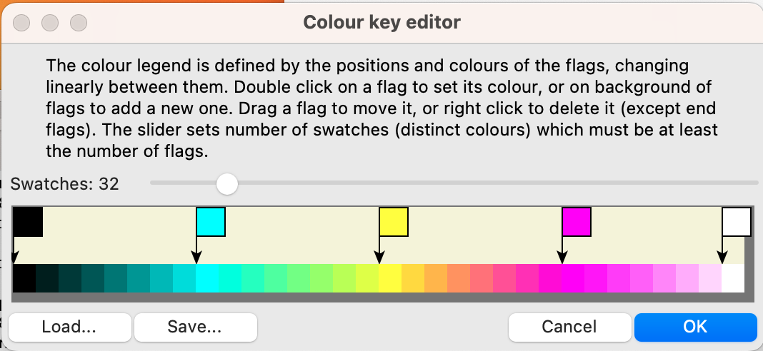
As well as editing the key as described in the dialogue, it can be loaded or saved in .rgb format, which is widely used by GIS systems. Simile's examples directory contains a saved legend, 'eightbit.rgb', which generates swatches corresponding to the colours that would be converted into each integer between 0 and 255 when using the 'eight-bit colourmap' option in the image data loader. It is thus possible to view an image which was loaded as data in a grid helper, possibly after it has been altered by execution of the model.
Running models : Working with visualisation tools : Plot value
Plot value against time helper
This is the classic time-plot helper. For most uses, it has been largely replaced by the Plotter helper.
It was not designed for presentation in a printed document, but for giving the model developer a robust, flexible display of how the value(s) for a single variable change over time. It automatically re-scales, on both the X (time) and Y axes, it can handle a variable no matter how deeply nested in multiple-instance submodels, and it displays the results from previous runs for comparison. It also gives the current values for all the variables in text form.
Each time you select a "Plot value against time" helper, you need to choose the variable to be plotted before the helper is displayed. You are alerted to this requirement by the message:
The following screen dumps show the standard ways this helper can be used.
This shows the value for a single-valued variable "size" from three successive runs of the model, using different parameter settings on each run. Note the automatic use of a different colour for each run, and the current value displayed at the bottom-left.
This shows the set of time plots for a single variable embedded inside a fixed-membership multiple-instance submodel. Since the number of instances is fixed for the duration of the run, we have the same number of lines throughout. Note that the line for each instance is different, reflecting the fact that each instance has different parameter values even though they all behave according to the same equations.
Here again we have the plot for a single run, for a single variable embedded inside a multiple-instance submodel. This time however the submodel is a population submodel, with individual instances coming into existence and disappearing during the course of the simulation run. Note then how lines start during the simulation (unlike the previous example, when all lines started at time zero), and also terminate during the course of the simulation, as individual instances are killed off. Each line has a different slope, reflecting the fact that the model was set up with a randomly-determined parameter value for each instance.
In: Contents >> Running models >> Working with helpers
Running models : Working with visualisation tools : Profiles
Time profiles helper
The time profiles helper is designed to show multiple attributes of each
instance of a population submodel. Each instance must be assigned a unique
identifier, which is plotted sequentially on the y-axis. A stacked bar
chart display is used to plot an arbitrary number of properties of that
instance against time.
For example, each individual in a population may hold wealth in the form
of property, stocks and shares, and cash. The time profiles helper will
display the changing wealth of each individual over time (the total height
of each bar) as well as the make-up of that wealth (the height of each
coloured segment).
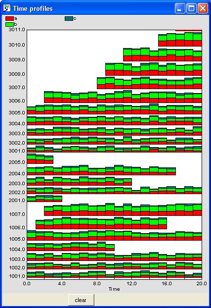
For best results, the variables plotted should be scaled to be less than
50. Panning and zooming operations are implemented as for the plotter helper. The y-axis can be panned up or down and
the x-axis panned left or right to display different parts of the axis at
the same magnification, whilst both axes can also be zoomed in or out to
increase or decrease the magnification.
-
 The cursor takes on the shape of a
four-headed arrow when placed over a scale point. Dragging a scale point
alters the range displayed by zooming in or out. To zoom in, drag the
scale points away from the origin, i.e. to the right (on the x-axis) or
upwards (on the y-axis). To zoom out, drag the scale points towards the
origin, i.e. to the left (on the x-axis) or downwards (on the y-axis).
-
 The cursor takes on the shape of a
two-headed arrow when placed over the axis itself. Dragging the axis
alters the range displayed by panning up or down, left or right.
In: Contents >> Running models >> Working with helpers
Running models : Working with visualisation tools : Model Explorer
Model Explorer
The model explorer provides a nested tree view of all the variables, compartments and flows used in the model. The elements are arranged by submodel, hierarchically from the top level desktop. In variable-membership submodels, additional elements used only in those submodels are also displayed. When a "helper" window requires a variable to be selected, this action can be performed by clicking on the required variable in the model explorer.
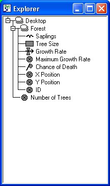
In: Contents >> Running models >> Working with helpers
Running models : Working with visualisation tools : Lollipop
Lollipop diagram helper
The "Lollipop diagram" is a means of displaying tree-like objects distributed in two dimensions. Each object has a size, which is used to calculate both the length of the trunk and branches. After invoking the helper, three variables are required for each component whose values are to be displayed, corresponding to the x-coordinates, the y-coordinates and the sizes. These can be variables or compartments, and are typically in a multiple-instance submodel. One tree then corresponds to each instance of the submodel.
Each set of values is displayed as trees of a diferent colour. A horizontal grid is also drawn, with x positions numbered in red, and y positions in blue. Numbers corresponding to heights of trees (z variable in the legend) are positioned above the grid corners in black.
There are sliders to adjust the longitude (view angle) and latitude (view elev.) of the point on an imaginary sphere surrounding the grid from which it is viewed. The image can be printed.
Note that all three variables can change through time, so although real-world trees may not move, their graphical representations can. This means the lollipop diagram helper can also be used for simulating animal movements, and so forth.
For best results, the x- and y-coordinates should be scaled between 0 and 100, and the size should be less than 25.
In: Contents >> Running models >> Working with helpers
Running models : Working with visualisation tools : Initialise
Standard helpers: Initial pseudo-random number generator
The functions rand_var() and rand_const() generate random numbers. For greater understanding of model behaviour it is sometimes convenient to generate the same (or the same sequence) of random numbers for several model runs. To do this, it is necessary to seed the random number generator with the same integer value each run. For this reason, they are known as pseudo-random numbers. A simple tool is provided to enter the seed.
To enter the seed:
- enter an integer value in the edit box;
- click on the "Set seed" button; and
- reset the model.
Note: It is important that the ![]() reset button on the "Run Control" is used AFTER initialising the pseudo-random number generator using the "Set seed" command. This is because some random numbers are generated when the model is reset.
reset button on the "Run Control" is used AFTER initialising the pseudo-random number generator using the "Set seed" command. This is because some random numbers are generated when the model is reset.
Example
Using the seed "123" will produce the following sequence of random numbers for the function rand_var(0,100) every time the simulation is performed:
62.3463, 2.2889, 13.6723, 11.7893, 92.8648, 56.7217, 93.8688, 96.4232, 96.3378, 75.1671, 49.0097, …
(At least if you are using the bundled MinGW C compiler under Windows. Other compilers may produce different sequences, owing to using different library implementations of the pseudorandom sequence generators, but this tool can still be used to achieve repeatability.)
In: Contents >> Running models >> Working with helpers
Running models : Working with visualisation tools : 3d
3d viewer helper
The 3d viewer helper is similar in operation to the spatial grid display helper, though four variables, rather than two, are required, to display the grid in three dimensions. These are, as before, the x-coordinates and the colours, but also, the y-coordinates and a sizes. Again, these are most commonly implemented using a fixed membership multiple-instance submodel.
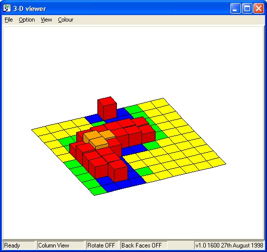
Amongst the many menu options, is the ability to switch to a surface view of the grid, as shown in the following screen shot. There are also options to rotate the graph through three dimensions, and to select the colours used.
In: Contents >> Running models >> Working with helpers
Other visualization tools : Event sounds helper
Other visualization tools : Event sounds helper
The motivation behind Simile's visualization tools is to provide the modeller with a continuous, immediate understanding of what the model is doing. Sometimes the best way to do this is with sounds rather than graphics. With the addition of discrete events to the modelling language, we realized that their instantaneous nature does not lend itself to the kind of graphical displays that work for continuous values.
So we created an event logger that also produces a sound each time a selected event occurs. Add an instance of this tool in the standard way, selecting 'Event sounds' from the list of helper titles. Now after clicking '+' in the helper window's toolbar, you can select a discrete event component in your model, and a sound file to play each time the event occurs. The window will show a 'ticker bar' which will move across the screen right to left, with a vertical line added each time the event occurs. Hovering over the lines will pop up the exact time and magnitude of the occurrence they represent.
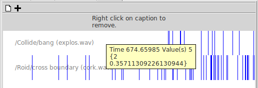
Also, the sound will be played each time the event occurs. If your event has a numeric magnitude, then the volume of the sound will be determined by where each event's magnitude falls between the min and max values given for the event. Sound files in WAV format will play on all platforms -- files in other formats (e.g., mp3) may play on your particular platform but are not guaranteed to play on all.
If the chosen event occurs very frequently, or if it is in a simple model that runs very fast, the sounds may overrun each other producing unpleasant noise. In this case you can use the 'limit updates/sec' feature to slow the model execution down to the point where the sounds can be heard separately.
Running models : Working with visualisation tools : Polygon diagram
Polygon diagram
This tool enables a dataset to be displayed as the colours of polygonal areas on a map. It can be used either where vector data for an actual map is available (either in the model, or in a separate file), or where an area is represented as some regular set of shapes whose vertices can be calculated by the model, e.g. hexagonal tiling.
A lot of the functionality of the polygon helper, including scrolling and zooming, working with the colour legend, and using it to edit model parameter values, is exactly the same as for the grid helper. However, the graphics of the polygon helper are not quite as fast, so you are more likely to need the 'freeze display' and 'manual update' features.
Loading co-ordinates from file
If you choose this option you will get a file selector to locate the data for the coordinates. If you choose a file with the extension .dxf, Simile will attempt to load it as a DXF file, and will then colour the polygons in the order in which they are defined in the file. Otherwise, Simile currently expects the file to contain all the X coordinates in nested list form, followed by all the Y coordinates. This is not particularly convenient, so we should add the option to set the coordinates from file using the table data dialogue too.
Loading co-ordinates from model
Of course you can put fixed parameters in the model and load them using the table data dialogue, then use them to set the boundaries of the polygons. If you choose this option, you will be asked to select model elements representing the X and Y coordinates of the polygon vertices. These elements should have two-dimensional data arrays, with the outer index being the number of the polygon whose border they define, and the inner index being the number of the vertex around that polygon. There should be the same number and arrangement of X and Y coordinates.
The usual way to get the coordinates is to have a submodel for the vertices inside the submodel representing the polygons. This should be a per-record submodel if different polygons have different numbers of vertices. Put fixed parameters for Xs and Ys inside the vertices submodel.
In: Contents >> Running models >> Working with helpers
Running models : Working with visualization tools : Edit sketch graph function
Standard helpers : edit sketch graph function
If your model contains equations that use the graph function, their function can be altered while the model is running. The tool for doing this appears as a helper, although it does not display values from the model or directly set them.
The helper is located in the "Standard tools" subdirectory menu and is called "Edit sketch graph function". Create an instance of the helper and click on the model component whose function you wish to alter. You will then see the same sketch graph editing window as when you originally created the sketch graph. You are able to drag the sketch line as well as edit the axis values and change the settings that control how the sketch is interpreted.
Any changes you make to the sketch graph function will take effect as soon as you hit the 'OK' button, but the helper will stay up until you delete it, allowing further changes to be made at any point. Note that the edited function will not be saved with the model. If you save the model after editing the sketch using the helper, it will keep the original version of the function. To change this you must go back to the equation dialogue and hit the "Graph" button.
Running models : Working with visualization tools : Data logger
The Data Logger tool does not display model data, but records it in files for later analysis with statistical tools. There are other ways of doing this:
- The Table Helper can save its contents as a .csv file, but has poor performance with large data sets
- The Snapshot tool can record values as the model runs, but only handles one variable, and needs setting up every time the model is run
By contrast, the Data Logger can handle any size of data set that is usable within Simile, and can log multiple variables, either in separate files or as columns in a single file. Since it is a standard helper, many instances can be added for different groups of values, and the setup can be saved as part of a general helper layout.
Using the tool
The tool's canvas will be blank when it is first added. To log a variable, hit the + button and click the variable on the model diagram. It will be listed within its hierarchy of submodels, with a '-' button ffor its removal. Hit + again to add more variables. The rightmost button in the helper's toolbar switches between saving separate files for each variable (named by the variable's caption) and a single file (log.csv) with each variable in its own column.
Saved file format
The helper will not save any data until you select a folder in which to save it. Click the toolbar button with the folder icon and navigate to the desired location. Now a line is written to the log file(s) at each display point as the model executes. The files are in .csv format with the time points stored in the left hand column. If the values being saved are arrays, they will be written as series of alternating indices and values, with each series enclosed in curly brackets, i.e., the same format as data popups or directly-entered file parameters.
The file is closed when the model is paused, and opened for appending more data when it is restarted. When the model is first run after a reset or rebuild, the file will be opened for writing, so the previous contents will be overwritten unless they have been moved.
As of Simile v6.9, it is also possible to log model data to a database -- either a file in some Excel-compatible format (.xls, .xlsx etc) or a MySQL database. To log to a database file, simply select it from the file dialogue. To log to a MySQL database, cancel the file dialogue and this will cause the database specification dialogue to appear. Here you enter the hostname, username, password and name of the MySQL database.
When logging to a database, each component being logged will have values put in its own column in the database. If logging an array component, there will be a separate column for each element in the array, named value/n where value is the name of the component and n is the index of the element. (value/n1/n2/... for multi-dimensional arrays). The values will be written to a table called 'Run 0' until the model is reset, after which new tables called 'Run 1', 'Run 2' etc will be created for data values from subsequent runs.
In: Contents >> Running models >> Working with helpers
Running models : Inspect model variable
 Inspect model variable
The snapshot tool is only available once a model has been built and is ready to run. It is provided to inspect the values of complex data structures held by some model elements. By hovering over a model variable it is possible to view pop-up windows that contain an element's equation, description and value. But in some cases, particularly where the data have more than one dimension, this pop-up window is rather hard to read. In any case, if the data is a very large array, the central portion will be elided to prevent the popup window being too large. As an alternative, use the snapshot tool. This will pop-up a larger, permanent window with the values structured by dimension.
As its name implies, the snapshot tool provides a view of the data structure at a moment in time. You can leave the window displaying the snapshot open, run the model for some more time, and then click again on the same element to open a second window that displays the new data structure. Having the two windows open at the same time, each labelled with the time at which the snapshot was taken, is the easiest way to trace changes to an element or sequence of elements. If you would rather just see the current data, the snapshot tool includes an update button ( ) which will refresh the displayed data with the current values from the model.
Saving data from snapshot tool
Normally you would use the data table helper to create a file containing model data. But because this tool is more oriented to displaying data interactively, it can operate very slowly with large tables. The snapshot tool is much quicker, although less flexible. Another alternative is to use the data logger helper, which is oriented towards storing data from many variables at once.
To save data from the snapshot tool at a given time point, hit the save button. It will prompt you for a file name and the data will be saved to this file as a comma-separated (.csv) file that can be loaded into a spreadsheet. The indices will be listed in columns to the left, outermost first, and the actual data items will appear in the rightmost column.
You can also use the snapshot tool to save data as a time series as the model runs. To do this, hit the log button ( ) and select a file name. Then start the model executing. The values displayed in the snapshot window will not change, but after each display interval the current values will be appended to the file. In this case the indices will be listed in rows at the top of the file, outermost first, with the actual data items appearing below them, one row for each time point. The times themselves will appear in the leftmost column. To stop logging, hit the log button again.
Remember that the snapshot tool is disabled until the model has been built. Only after building the model do the elements have values. The tool is available at any point during the model run.
Parameter estimation using PEST
Parameter estimation using PEST
PEST is an advanced software tool for model calibration, parameter estimation and predictive uncertainty analysis. It is open-source and freely available, and currently distributed by S. S. Papadopoulos & Associates, Inc.
You will need to install PEST separately on your computer, and ensure that it can be executed from the command line. How to install PEST
PEST communicates with Simile models by creating files containing parameter values, running the model then reading files containing model output values. The model will be run many times. How to set up PEST interaction
When using PEST, model inputs and outputs can be individual values or sequences over time. If an output is a time series, the series itself can be plotted on a display tool alongside the model output. Running PEST
Predictive analysis can be used to get an estimate of a model output at a time later than that covered by available data, or it can be used to provide an uncertainty band around a model output trace. Working with predictive analysis
In: Contents >> Running models
How to install PEST
How to install PEST
PEST is an advanced software tool for model calibration, parameter estimation and predictive uncertainty analysis. It is open-source and freely available, and currently distributed by S. S. Papadopoulos & Associates, Inc. The Simile interface has been verified to work with PEST version 9 and later, on Windows, Linux and MacOS.
Windows users can download a pre-compiled version of PEST from this site and follow the instructions to enable it to run from the command line. Typing 'pest' to the command prompt will produce a message about usage if it is correctly installed.
Linux and Mac users will need to compile PEST from source. PEST is written in FORTRAN, and the GNU g95 compiler is suitable for compiling it. This is part of the GNU compiler collection, and is freely available from SourceForge. Some Linux distributions have the gfortran extension to gcc available from their software repositories, which is also suitable for compiling PEST.
It should be possible to build the package using the makefile shipped with it. The simplest way to get this to work is to create a symlink called 'f90' to the g95 compiler, since the makefiles all include f90 as the default compiler name. This can be placed in a directory in the executable search path, e.g., ~/bin. A symlink to the PEST executable can also be made in this directory once it is compiled.
Check that PEST is installed correctly by typing 'pest' to the command prompt before attempting to run it from within Simile. If it is set up correctly, it will generate a usage help message.
In: Contents >> Running models >> PEST
Setting up PEST interaction
Setting up PEST interaction
Once you have got your model behaving in a generally believable way, you can use PEST to calibrate your model parameters in order to match the model's output to a set of measured data.
Details of the operation of PEST can be found in its manual. The manual is included in the pre-compiled Windows distribution. Only the basics of PEST operation will be covered here.
The PEST interface is included in Simile as a helper. It is located in the 'Standard tools' submenu of the helpers menu. When you select it, it will create a tabbed notebook with four pages inside its top-level window. These are labelled Inputs, Outputs, Actions and Settings. If using the single-window Model Run Environment, be careful not to confuse these notebook tabs with those containing other helper pages.
Inputs
On this page you specify which model parameters will be estimated by PEST. You can add a single parameter by hitting the '+' button at the top, then clicking on the parameter in the model diagram or explorer tool. The '-' button allows you to remove a parameter. The last button adds all suitable parameters that have not already been added. Note that PEST can only optimize real (floating-point) value parameters.
A minimum and maximum value must be provided for each parameter. For fixed parameters you can type these into entry boxes. They must reflect the range of values which are plausible. For variable parameters, PEST uses the values entered in the parameter's properties before the model was built.
For variable parameters you can decide whether PEST simply picks a fixed value for them or generates a series of values. There is a checkbox and an entry field for your choice. A series will be spaced regularly over the length of the model run, which is specified in the Actions page. Note that the total number of values being estimated (including all members of each array and each series) must not exceed the number of data measurements being used, or PEST will not have enough information to estimate them all.
PEST also needs an initial estimate for each parameter value. This defaults to midway between the parameter's minimum and maximum value, but you can enter a different estimate. If you select the 'Use current data as estimates' checkbutton at the bottom of the Inputs page, PEST will use the current values at the start of the optimization for its initial estimates.
If an array parameter is used, PEST will use the same specification data for each array member, but will create a separate estimate for each member.
Outputs
On this page you specify which model values are to be looked at by PEST and compared with measured values. Any value in the model can be used, except values from inside variable-membership submodels. You can add a value by hitting the '+' button at the top, then clicking on the value in the model diagram or explorer tool. This indicates a component whose value at the end of each model run is to be compared with measured data. You can also add a value by hitting the graph icon button. This indicates a component whose value is to be sampled at a series of time points during a model run, and each sample compared with measured data. The '-' button allows you to remove a value of either type.
For each value you also need to load measurement data for comparison. PEST displays an input tool similar to the one in the 'File Parameters' dialogue, and data can be entered directly or loaded from files exactly as described for this dialogue.
When you have loaded your measurement data you can save references to it in a scenario file, as you would for parameter data. This scenario file will have the extension .smf rather than .spf to indicate that it refers to measurement data rather than parameter data. In other respects the two file formats are interchangeable.
Restrictions
Simile is a much mode expressive modelling tool than the typical command-line-driven models with which PEST is intended to work, so there are some limits on what Simile model constructs can be used when estimating parameters with PEST. In particular,
- The interface does not support multidimensional data arrays, or any arrays that are supplied or sampled at different time points since this effectively involves a multidimensional array.
- Data values must be real, and array indices must be integer (i.e., not enumerated-type).
In: Contents >> Running models >> PEST
Running PEST
Running PEST
When you have set up the inputs and outputs in your model that will be used by PEST, you can go the the Actions tab in the PEST interface tool notebook and try to run it.
The run length from the run control will be used unless you alter it in the input box. If you do not select the checkbox in the Predictive analysis section, a simple parameter estimation will be done. Note that if all your outputs are time series, the run length will be up to the last time series value and the entry box for it will have no effect.
A PEST run can be controlled in the same way as a model run
While PEST is running you will see the run control values and progress bar update during each run. You will also see statistics about the run appear in the execution monitor box of the Actions tab. The text box in the execution monitor displays PEST's output to the command line, which is useful in case it should fail for any reason.
Simile's other helper tools are also updated while PEST runs. This means that if you have a slider tool for the variable parameters which are under PEST's control, you can watch them update as PEST adjusts them to optimize the outputs. However you may not want the tools to be updated, as they may slow down execution, and the plotter will show a separate trace for each run. To turn off all helper updates, set the 'Display interval' entry in the Run Control dialogue to zero. Alternatively you can set it to an interval longer than the run length, so the helpers (including sliders) will only be updated at the start of each run.
When PEST has finished optimizing, the model's parameters will be set to the values it has estimated. You can now go to the file parameters dialogue and save these values in a scenario file if they will be required later. PEST provides an indication (the 'phi' value) of how good its estimation is, and this is reported in the Actio tab of the helper -- the lower the phi value, the better the estimation. For a graphical view, if you have a time series of measurements and you are displaying the corresponding model value on a tool such as the plotter, you can select the 'show these values on plots' checkbox at the bottom of the PEST tool Outputs panel, then reset and run the model again, and a trace of the measured data will be superposed on the model data trace in the plotter tool.
PEST produces a selection of output files during a run. These are kept in Simile's temporary directory. When PEST has finished running, you can save any of these in a permanent directory using the 'Save a PEST file...' button. Each pest file has a different extension; use the extension chooser in the save dialogue to choose the file you want, and enter the name you want to give it.
If PEST fails to converge on a good set of parameters, you can adjust its settings. The global settings, such as NOPTMAX to control the maximum allowed number of optimization stages, are on the Settings tab. Settings related to each input or output, such as PARCHGLIM which affects how the maximum change of an input value on a single step is applied, can be edited in a context menu for that input or output
In: Contents >> Running models >> PEST
Predictive analysis
Predictive analysis
When you first run PEST, it runs in parameter estimation mode. This selects values for the input parameters which cause the outputs to most closely follow the measured values, according to the least-squares rule. The quality of fit is given by PHI
The purpose of predictive analysis is to determine the range over which a model output can vary while still being consistent with the measured values supplied. To get maximum and minimum predictions, PEST allows the PHI value to be larger than the minimum value found during parameter estimation.
To do a predictive analysis on a Simile model, check the checkbox in the predictive analysis frame on the Actions tab, and select a model value for which to make a prediction. This can be any non-parameter value in the model, not including those in variable-membership submodels. It can be a value which you are already using for comparison with measured data
You can also make the following selections:
-
Whether to predict maximum or minimum values
-
What multiple of the original PHI to allow for the predictions
-
At what time(s) the prediction will apply.
There are some values on the Settings tab which affect PEST's behaviour during predictive analysis; these are explained in the PEST manual. Simile supplies default values for these, based on the results obtained when running PEST in parameter estimation mode.
If the value being predicted is an array, or if the frequency and duration you set for prediction times are such that a prediction will be made at more than one time, then a complete run of PEST must be done for each prediction, because PEST itself can only predict one value at a time. Since each PEST run includes multiple model runs, predicting large numbers of values can take a very long time. The following steps might speed things up:
-
Set display interval to 0, so display tools do not take up time
-
Select 'use current values as estimates' on the Inputs tab after the parameter estimation run, so each prediction run starts with good parameter estimates.
During a prediction run, the progress bar shows how many of the prediction runs have been completed. Predicted values will be inserted into the results field, and can be displayed in tabular form and saved as a .csv file using the View button.
It is worth noting that each prediction is arrived at independently. So, if using predictive analysis to create 'error bands' around a graph of model outputs, it might be the case that although each individual value might vary as far as the predicted limits, it would be impossible for the graph line to actually follow the minimum or maximum limits, since multiple predicted values on the limit might be incompatible with each other. Remember, however clever PEST might appear, it's still only a computer program.
In: Contents >> Running models >> PEST