Modelling predator-prey interactions
Introduction
The classic, textbook predator-prey model is that proposed by Lotka and Volterra in 1927. In words, the model states that:
- Each prey gives rise to a constant number of offspring per year;
In other words, there are no other factors limiting prey population growth apart from predation. - Each predator eats a constant proportion of the prey population per year;
In other words, doubling the prey population will double the number eaten per predator, regardless of how big the prey population is. - Predator reproduction is directly proportional to prey consumed;
Another way of expressing this is that a certain number of prey consumed results in one new predator; or that one prey consumed produces some fraction of a new predator. - A constant proportion of the predator population dies per year.
In other words, the predator death rate is independent of the amount of food available.
Mathematically, the model is conventionally expressed as:
dX/dt = aX - bXY
dY/dt = cbXY - dY
where:
X = size of the prey population (set to an initial value of 5000 in this tutorial);
Y = size of the predator population (45);
a = number of offspring per prey per year (set to 0.5 in this tutorial);
b = proportion of the prey population consumed by one predator per year (0.01);
c = conversion of one prey consumed into new predators (0.01, i.e. 100 rabbits eaten gives rise to one new fox);
d = proportion of predator population dying per year (0.2).
At the end of this tutorial, we will see how to implement the conventional form of the model, exactly as given. However, we will begin by building up a population model for a single species in System Dynamics terms, then add the predator population, then show how one of the relationships can be made more biologically realistic, before returning to the conventional form of the model.
Stage 1: Modelling the dynamics of a single population
| Step 1 |
Add two
 compartments to the desktop, and rename them rabbits and foxes compartments to the desktop, and rename them rabbits and foxes |
| Step 2 |
Draw a
 flow into the rabbits compartment, and rename it rabbit repro flow into the rabbits compartment, and rename it rabbit repro |
| Step 3 |
Draw a
 flow out of the rabbits compartment, and rename it predation flow out of the rabbits compartment, and rename it predation |
| Step 4 |
Draw an influence arrow from:
|
| Step 5 |
Enter the following expression for the rabbit repro flow: 0.5*rabbits
|
| Step 6 |
Enter the following expression for the predation flow: 0.01*rabbits*foxes
|
| Step 7 |
Set the initial value for the rabbits compartment to 5000
|
| Step 8 |
Set the initial value for the foxes compartment to 45
|
| Step 9 |
“Build” the model.
|
| Step 10 |
Change the Run Control settings:
|
| Step 11 |
Set up a plotter display for the rabbits compartment.
|
| Step 12 |
Run the model
Note that the population grows exponentially — there is nothing to hold it in check. |
Stage 2: Adding in predator dynamics
| Step 1 |
Add a
 flow into the foxes compartment, and rename it fox repro. flow into the foxes compartment, and rename it fox repro. |
| Step 2 |
Add a
 flow out of the foxes compartment, and rename it fox mortality. flow out of the foxes compartment, and rename it fox mortality. |
| Step 3 |
Draw an
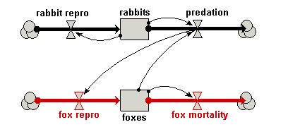
 influence from the rabbit’s predation flow to the fox repro flow. influence from the rabbit’s predation flow to the fox repro flow.This reflects the assumption in the standard textbook model, that the predator reproduction is proportional to rate of predation on the prey. Your model diagram should now look like this:
|
| Step 4 |
Enter the following expression for the fox repro flow: 0.01*predation
|
| Step 5 |
Enter the following expression for the fox mortality flow: 0.2*foxes
|
| Step 6 |
Rebuild the model
|
| Step 7 |
Set up
 graph display for the foxes compartment graph display for the foxes compartmentNote that you need to have a separate plotter display, since the number of foxes is typically a couple of orders of magnitude less than the number of rabbits. If you plotted them on the same graph, the graph line for the number of foxes would be right on the X axis. |
| Step 8 |
Run the model again
You should now see that the rabbits and the foxes compartments cycle, with the rabbits population crashing as the foxes population increases, followed by a crash in the foxes population. |
Stage 3: Re-casting the model diagram
The present model is based on a number of assumptions that are biologically unsound. For example, it assumes that the number of rabbits eaten per fox is directly proportional to the number of rabbits, so doubling the number of rabbits doubles the number eaten per fox — even if there are millions of rabbits around!
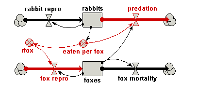
We will tackle the problem of making the model more biologically realistic in two stages. First, we will change the model diagram a little, adding in a couple of variables and changing the influence arrows, but retaining the same mathematical structure: the revised model should produce exactly the same results. These changes provide more appropriate handles in our model for expressing biologically-meaningful relationships. Then, in the following stage, we will replace some of the simplistic assumptions in this model with others that are biologically more realistic.
| Step 1 |
Use the
 delete tool to remove the influence arrows from rabbits to predation, and from predation to fox repro. delete tool to remove the influence arrows from rabbits to predation, and from predation to fox repro. |
| Step 2 |
Add in two new
 variables, naming them rfox and eaten per fox. variables, naming them rfox and eaten per fox. |
| Step 3 |
Draw
 influence arrows: influence arrows:
Your model diagram should now look like this:
|
| Step 4 |
Enter the following expression for each variable or flow:
Satisfy yourself that these changes have not altered the mathematical nature of the model. |
| Step 5 |
Re-build and run the model again, confirming that you do indeed get the same behaviour that you had before.
|
Stage 4: Sketching biologically meaningful relationships
What we now have are some variables in our model ( and ) for introducing biologically-meaningful relationships. The influence arrows we have drawn to these two variables expresses the biologically-reasonable assumptions that:
- the number of rabbits eaten per fox, , depends on the number of rabbits; and
- the number of baby foxes produced per fox, , depends on the number rabbits eaten per fox.
So far, however, we have retained the simplistic assumptions from the conventional model: we have asumed that the number of rabbits eaten per fox is directly proportional to the number of rabbits; and that the rate of reproduction per fox is directly proportional to the number of rabbits eaten. In reality, both assumptions are way off the mark: if there are lots of rabbits around, then foxes reach a limit of how many they can eat. Similarly, even if foxes succeed in eating many rabbits, there is an upper limit to the number of offspring they can produce per year.
How can we incorporate these refinements?
We have two options. One is to find some mathematical expression that better captures our understanding. If you are mathematically inclined, you might like to give that a try. The other is to exploit Simile’s ability to draw a sketch graph of any relationship between two variables, and that’s what we’ll do here.
| Step 1 |
Open up the Equation dialogue window for the variable eaten per fox, and delete the existing expression.
|
| Step 2 |
Click on the
 graph button graph buttonThis opens up a separate graph pad window.
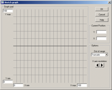
The scaling for each axis is determined by the Xmin, Xmax and Ymin, Ymax edit boxes. The graph pad area (initially a horizontal line running through the middle of the graph pad) which can be adjusted up and down using the mouse. |
| Step 3 |
Scale the X axis (representing number of rabbits), by entering a value of 10000 in the Xmax edit box at the right of the X axis.
|
| Step 4 |
Scale the Y axis (number of rabbits eaten per fox per year), by entering a value of 100 in the edit box at the top of the y axis.
|
| Step 5 |
Move the mouse into the graphpad area, and move the mouse around while holding down the mouse button.
Notice how you can adjust the position of the line showing the relationship between the Y and X axes. |
| Step 6 |
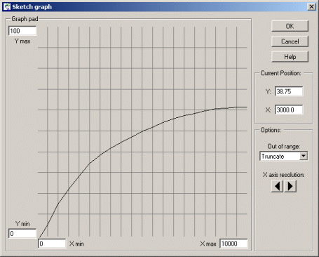
Adjust it so that it passes through the origin at (0,0), and rises up smoothly till it reaches a plateau (asymptotic) value, looking something like this:
When Simile comes to run the model, it will use linear interpolation to work out what the value on the Y axis is knowing the value on the X axis. |
| Step 7 |
Click on the Enter button to close the sketch graph window.
|
| Step 8 |
In the main Equation window, Simile has entered the text graph( ) into the equation field. Insert the name of the rabbits compartment between the brackets, so that the expression now read: graph(rabbits)
|
| Step 9 |
Open up a graph pad in the Equation dialogue window for the variable rfox, and delete the existing expression.
We are now going to sketch the relationship between , the number of foxes produced per fox per year, and , the number of rabbits eaten per fox per year. |
| Step 10 |
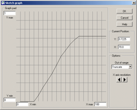
Scale it, setting Xmax to 100 and Ymax to 1.
Note that the Xmax value (100) is the same as the Ymax value in the previous sketch graph. This is because they actually refer to the same variable: number of rabbits eaten per fox per year. The value of 1 for the Y axis indicates that foxes cannot produce more than 2 baby foxes per year. |
| Step 11 |
Sketch a graph looking something like this:
Before reading the rest of this comment, try to figure out for yourself what this is saying... It shows that a fox does not reproduce at all when its food intake is below some lower threshold. After that, its rate of reproduction is directly proportional to the amount of additional food consumed, up to some maximum, plateau level: the maximum number of young it can produce per year. |
| Step 12 |
Click on the Enter button to close the sketch graph window.
|
| Step 13 |
Edit the expression so that it reads graph(eaten_per_fox).
Note that the variable whose label is (with spaces between the words) is written as eaten_per_fox in the equation. This is because some characters which are allowed in labels are not allowed in variables in expressions. Note that Simile always lists the influencing variables at the bottomof the Equation window, so you can always check on what spelling it’s using. |
| Step 14 |
Rebuild the model, and run it again.
You should notice a difference in the shape of the graphs, reflecting the changes in the model. |
Stage 5: Bonus section: re-visiting the classic predator-prey model.
In this tutorial, I began by sticking faithfully to the mathematical form of the traditional Lotka-Volterra predator-prey model, but I designed the System Dynamics diagram to put more emphasis on biological processes. Thus, I used four flow arrows, representing reproduction and mortality processes for the two populations, even though these were not explicitly mentioned in the original model: all we had were two rate-of-change equations. This reflects my personal attitude to modelling, that it should begin as a conceptual design activity, rather than being driven by mathematical notation.
Nevertheless, there will be times when you come across a model expressed as a set of differential equations, and you feel you have neither the inclination nor ability to re-express it in terms of biological process, represented as separate flows. What can you do?
Well, it’s really pretty straightforward All you have to do is to follow these four simple steps:
- Create one compartment for each state variable
- Make a single inflow for each compartment
- Draw influence arrows from compartments to inflows, as required by the differential equations.
- Enter each differential equation into the flow for the corresponding state variable
Let’s see this in action:
| Step 1 |
Start a new model.
|
| Step 2 |
Add two compartments, and re-label them X and Y respectively.
|
| Step 3 |
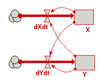
Add a single flow into each compartment, and re-label them dXdt and dYdt respectively.
|
| Step 4 |
Draw influence arrows from both compartments to both flows (i.e. four arrows in total).
Your model diagram should now look like this:
|
| Step 5 |
Enter the following expressions into the flows:
|
| Step 6 |
Build and run the model!
|
Your model diagram should now look like this: